Gregory’s forcing-feedback regression (2004)

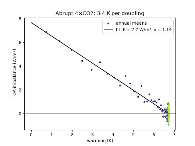
Jonathan Gregory and colleagues proposed a way to read forcing and feedback from a single run in which CO2 is quadrupled abruptly. Each year the net top-of-atmosphere imbalance N = F - lambda T is plotted against the warming. The intercept is the forcing, the slope is minus the feedback, and the line crosses zero at the equilibrium warming, without running to equilibrium. Here the run is a one-box model with seeded annual noise added to the imbalance.

import matplotlib.pyplot as plt
import numpy as np

from earthsciencekit.climate import equilibrium_warming, gregory_regression, simulate_one_box
from earthsciencekit.units import convert

forcing, restoring, capacity = 7.4, 1.1, 3e8
years = np.arange(0, 151)
warming = simulate_one_box(forcing, restoring, capacity, convert(years, "year", "s")).values[:, 0]
imbalance = forcing - restoring * warming
np.testing.assert_allclose(gregory_regression(warming, imbalance), [forcing, restoring])
noisy = imbalance + np.random.default_rng(2004).normal(0, 0.4, years.size)
fitted_forcing, fitted_restoring = gregory_regression(warming[1:], noisy[1:])
assert np.isclose(fitted_forcing, forcing, rtol=0.1) and np.isclose(fitted_restoring, restoring, rtol=0.1)
sensitivity = equilibrium_warming(fitted_forcing / 2, fitted_restoring)

line = np.linspace(0, fitted_forcing / fitted_restoring, 2)
fig, ax = plt.subplots()
ax.scatter(warming[1:], noisy[1:], c=years[1:], s=10, cmap="viridis", label="annual means")
ax.plot(line, fitted_forcing - fitted_restoring * line, "k", label=f"fit: F = {fitted_forcing:.1f} W/m², λ = {fitted_restoring:.2f}")
ax.axhline(0, color="0.5", lw=0.8)
ax.set(xlabel="warming [K]", ylabel="TOA imbalance [W/m²]", title=f"Abrupt 4×CO2: {sensitivity:.1f} K per doubling")
ax.legend()

plt.show()