Kelvin’s conduction on a discrete grid

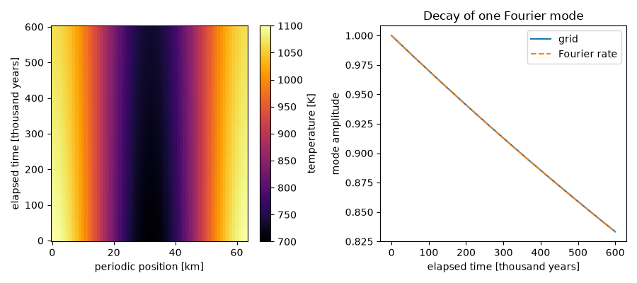
Kelvin’s calculation rests on Fourier’s conduction law, under which every sinusoidal temperature mode decays at the rate kappa k**2. On a periodic grid the same mode decays at 4 kappa sin(k dx / 2)**2 / dx**2, which tends to Fourier’s rate as the grid is refined, and the mean temperature is conserved because no heat leaves a periodic domain.

import matplotlib.pyplot as plt
import numpy as np

from earthsciencekit.plate_tectonics import diffuse_temperature
from earthsciencekit.units import convert

n, spacing, diffusivity = 64, 1000.0, 1e-6
x = np.arange(n) * spacing
k = 2 * np.pi / (n * spacing)
initial = 900 + 200 * np.cos(k * x)
time = convert(np.linspace(0, 0.6e6, 101), "year", "s")
result = diffuse_temperature(initial, time, diffusivity, spacing)
np.testing.assert_allclose(result.values.mean(axis=1), 900, atol=1e-10)
amplitude = (result.values[:, 0] - 900) / 200
assert np.isclose(-np.log(amplitude[-1]) / time[-1], diffusivity * k**2, rtol=1e-3)

fig, (left, right) = plt.subplots(1, 2, figsize=(9, 4))
image = left.pcolormesh(x / 1e3, convert(time, "s", "year") / 1e3, result.values, shading="auto", cmap="inferno")
left.set(xlabel="periodic position [km]", ylabel="elapsed time [thousand years]")
fig.colorbar(image, ax=left, label="temperature [K]")
right.plot(convert(time, "s", "year") / 1e3, amplitude, label="grid")
right.plot(convert(time, "s", "year") / 1e3, np.exp(-diffusivity * k**2 * time), "--", label="Fourier rate")
right.set(xlabel="elapsed time [thousand years]", ylabel="mode amplitude", title="Decay of one Fourier mode")
right.legend()
fig.tight_layout()

plt.show()