Sverdrup’s balance (1947)

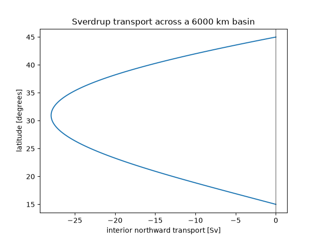
Harald Sverdrup showed that in the ocean interior the curl of the wind stress is balanced by flow across lines of latitude, where the planetary vorticity changes at the rate beta. Under the westerlies and trade winds of a subtropical gyre the whole interior drifts equatorward by tens of Sverdrups, and a narrow current on one boundary must carry it back.

a 100 km wide, 1000 m deep boundary current must flow at 0.28 m/s

import matplotlib.pyplot as plt
import numpy as np

from earthsciencekit.constants import EARTH_RADIUS, OMEGA_EARTH
from earthsciencekit.oceanography import sverdrup_transport, volume_transport
from earthsciencekit.units import convert

stress, width, south, north = 0.1, 6000e3, np.radians(15), np.radians(45)
length = EARTH_RADIUS * (north - south)
latitude = np.linspace(south, north, 121)
y = EARTH_RADIUS * (latitude - south)
curl = -stress * np.pi / length * np.sin(np.pi * y / length)
beta = 2 * OMEGA_EARTH * np.cos(latitude) / EARTH_RADIUS
interior = convert(sverdrup_transport(curl, 1025, beta) * width, "m^3/s", "Sv")
assert -60 < interior.min() < -10

return_speed = -interior.min() * 1e6 / (100e3 * 1000)
assert np.isclose(convert(volume_transport(return_speed, 100e3, 1000), "m^3/s", "Sv"), -interior.min())
print(f"a 100 km wide, 1000 m deep boundary current must flow at {return_speed:.2f} m/s")

fig, ax = plt.subplots()
ax.plot(interior, np.degrees(latitude))
ax.axvline(0, color="k", lw=0.5)
ax.set(xlabel="interior northward transport [Sv]", ylabel="latitude [degrees]", title="Sverdrup transport across a 6000 km basin")

plt.show()