Gustafson and Kullenberg’s inertial oscillations (1936)

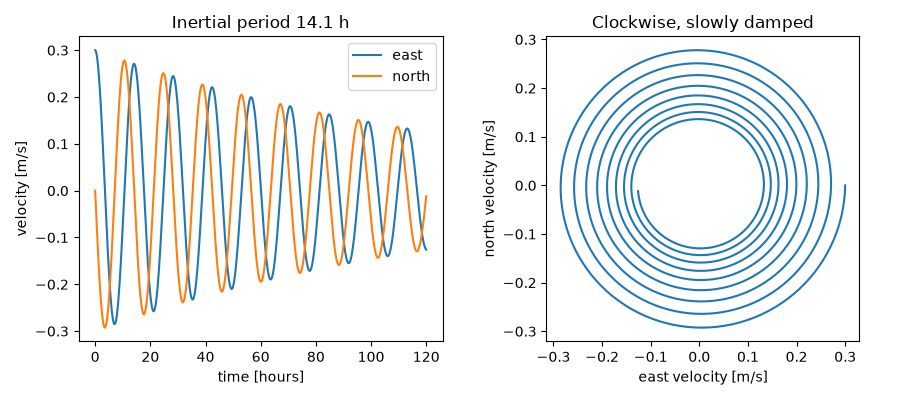
Torsten Gustafson and Börje Kullenberg moored current meters in the Baltic off Gotland and found currents turning clockwise with a period of about 14 hours. That is the inertial period 2 pi / f at 57.8 N: once the wind stops, water keeps moving and the Coriolis force turns it in circles that friction slowly damps.

import matplotlib.pyplot as plt
import numpy as np

from earthsciencekit.atmosphere import coriolis_parameter
from earthsciencekit.oceanography import inertial_period, simulate_inertial_current

f = coriolis_parameter(np.radians(57.8))
period = inertial_period(f)
assert np.isclose(period / 3600, 14.2, atol=0.1)

time = np.linspace(0, 5 * 86400, 2001)
result = simulate_inertial_current(f, time, east_speed=0.3, damping=2e-6)
east = result.values[:, 0]
upward = np.flatnonzero((east[:-1] < 0) & (east[1:] >= 0))
assert np.isclose(np.mean(np.diff(time[upward])), period, rtol=0.01)
assert result.values[1, 1] < 0  # clockwise: an eastward current first turns south

fig, (left, right) = plt.subplots(1, 2, figsize=(9, 4))
left.plot(time / 3600, result.values, label=["east", "north"])
left.set(xlabel="time [hours]", ylabel="velocity [m/s]", title=f"Inertial period {period / 3600:.1f} h")
left.legend()
right.plot(*result.values.T)
right.set(xlabel="east velocity [m/s]", ylabel="north velocity [m/s]", aspect="equal", title="Clockwise, slowly damped")
fig.tight_layout()

plt.show()