Dziewonski and Anderson’s PREM (1981)

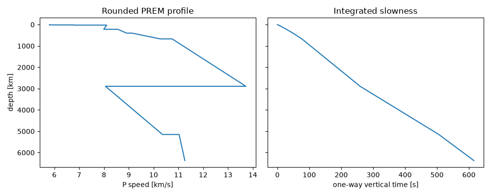
Adam Dziewonski and Don Anderson fitted one spherically symmetric Earth model, PREM, to travel times, normal modes and the Earth’s mass and moment of inertia. Integrating slowness through such a table predicts arrival times. The rounded P-wave values below follow PREM. A vertical ray from the surface through the centre to the antipode takes about 20 minutes, close to the tabulated PKIKP time of about 1212 s.

surface to antipode: 1231 s; to the core: 259 s

import matplotlib.pyplot as plt
import numpy as np

from earthsciencekit.seismology import vertical_travel_time

depth_km = np.array([0, 15, 15, 24.4, 24.4, 220, 220, 400, 400, 670, 670, 2891, 2891, 5150, 5150, 6371])
vp_km_s = np.array([5.8, 5.8, 6.8, 6.8, 8.11, 7.99, 8.56, 8.91, 9.13, 10.27, 10.75, 13.72, 8.06, 10.36, 11.03, 11.26])
time = vertical_travel_time(depth_km * 1e3, vp_km_s * 1e3)
antipode = 2 * time[-1]
assert np.isclose(antipode, 1212, rtol=0.03)
print(f"surface to antipode: {antipode:.0f} s; to the core: {time[11]:.0f} s")

fig, axes = plt.subplots(1, 2, figsize=(10, 4), sharey=True)
axes[0].plot(vp_km_s, depth_km)
axes[0].set(xlabel="P speed [km/s]", ylabel="depth [km]", title="Rounded PREM profile")
axes[1].plot(time, depth_km)
axes[1].set(xlabel="one-way vertical time [s]", title="Integrated slowness")
axes[0].invert_yaxis()
fig.tight_layout()

plt.show()