Mahaffy’s shallow-ice model (1976)

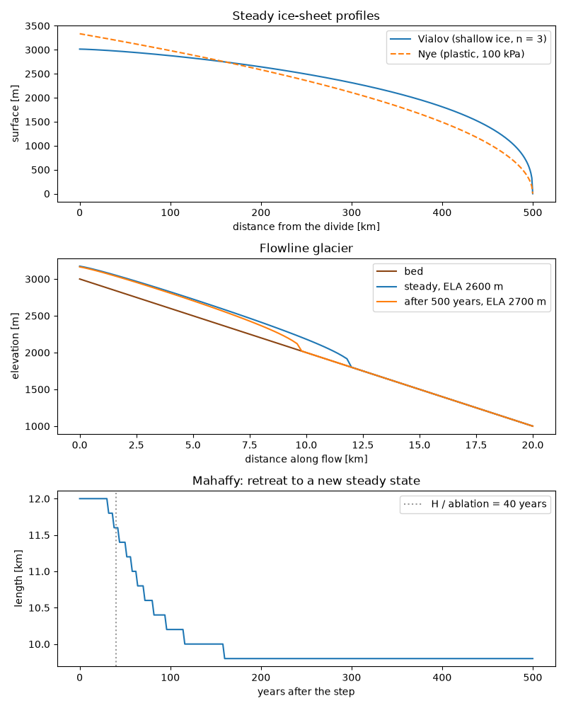
M. W. Mahaffy built the first three-dimensional numerical ice-sheet model, for the Barnes Ice Cap. Because ice sheets are thin, the flux at each point follows from the local thickness and surface slope, and the thickness obeys a nonlinear diffusion equation solved on a staggered grid. Its steady state on a flat bed is Vialov’s (1958) profile, flatter at the dome than Nye’s parabola. simulate_flowline_glacier applies the same scheme to a mountain glacier, here grown on a bare bed and then shown responding to a 100 m rise of its equilibrium line.

import matplotlib.pyplot as plt
import numpy as np

from earthsciencekit.constants import GRAVITY, ICE_DENSITY, SECONDS_PER_YEAR
from earthsciencekit.glaciology import (
    glacier_response_time,
    nye_plastic_profile,
    simulate_flowline_glacier,
    vialov_dome_height,
    vialov_profile,
)

half_width = 500e3
dome = vialov_dome_height(half_width, 0.3 / SECONDS_PER_YEAR, 2.4e-24, 3, ICE_DENSITY, GRAVITY)
distance = np.linspace(0, half_width, 501)
x = np.arange(0, 20e3 + 1, 200.0)
bed = 3000 - 0.1 * x
gradient = 0.007 / SECONDS_PER_YEAR
spin_up = simulate_flowline_glacier(bed, 200.0, 2600.0, gradient, np.linspace(0, 1500, 76) * SECONDS_PER_YEAR)
steady = spin_up.values[-1, 2:]
years = np.linspace(0, 500, 251)
step = simulate_flowline_glacier(bed, 200.0, 2700.0, gradient, years * SECONDS_PER_YEAR, initial_thickness=steady)
terminus = steady[steady > 1][-1]
tau = glacier_response_time(steady.max(), gradient * (2600 - bed[np.count_nonzero(steady > 1)])) / SECONDS_PER_YEAR
area = step.values[:, 1]
assert area[-1] < area[0] and abs(area[-1] - area[-2]) < 1e-6 * area[0] and terminus > 0

fig, (top, middle, bottom) = plt.subplots(3, 1, figsize=(8, 10))
top.plot(distance / 1e3, vialov_profile(distance, half_width, dome, 3), label="Vialov (shallow ice, n = 3)")
top.plot(distance / 1e3, nye_plastic_profile(half_width - distance, 1e5, ICE_DENSITY, GRAVITY), "--", label="Nye (plastic, 100 kPa)")
top.set(xlabel="distance from the divide [km]", ylabel="surface [m]", title="Steady ice-sheet profiles")
top.legend()
middle.plot(x / 1e3, bed, color="saddlebrown", label="bed")
middle.plot(x / 1e3, bed + steady, label="steady, ELA 2600 m")
middle.plot(x / 1e3, bed + step.values[-1, 2:], label="after 500 years, ELA 2700 m")
middle.set(xlabel="distance along flow [km]", ylabel="elevation [m]", title="Flowline glacier")
middle.legend()
bottom.plot(years, step.values[:, 0] / 1e3)
bottom.axvline(tau, color="0.6", ls=":", label=f"H / ablation = {tau:.0f} years")
bottom.set(xlabel="years after the step", ylabel="length [km]", title="Mahaffy: retreat to a new steady state")
bottom.legend()
fig.tight_layout()

plt.show()