Morton, Taylor and Turner’s buoyant plumes (1956)

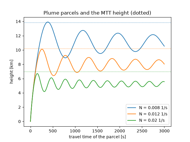
Morton, Taylor and Turner assumed that a turbulent plume draws in surrounding fluid at a speed proportional to its own rising speed. Three flux equations then describe it, and in a stably stratified fluid the plume rises to a height of about 5.0 F**(1/4) N**(-3/4) set by only its buoyancy flux and the stratification. Following a parcel up the axis shows the rise, the top and the fall back towards the level of neutral buoyancy, where the plume spreads. A vent of finite size tops out a few percent below the point-source height.

import matplotlib.pyplot as plt
import numpy as np

from earthsciencekit.volcanology import plume_rise_height, simulate_eruption_column

radius, velocity, buoyancy = 100.0, 100.0, 30.0
flux = radius**2 * velocity * buoyancy
time = np.linspace(0, 3000, 1501)
fig, ax = plt.subplots()
for frequency in [0.008, 0.012, 0.02]:
    result = simulate_eruption_column(radius, velocity, buoyancy, frequency, time)
    top = plume_rise_height(flux, frequency)
    assert np.isclose(result.values[:, 0].max(), top, rtol=0.05)  # a finite vent sits a few percent below the point source
    (line,) = ax.plot(time, result.values[:, 0] / 1e3, label=f"N = {frequency} 1/s")
    ax.axhline(top / 1e3, color=line.get_color(), ls=":", lw=1)
ax.set(xlabel="travel time of the parcel [s]", ylabel="height [km]", title="Plume parcels and the MTT height (dotted)")
ax.legend()

plt.show()