Ricker’s wavelet (1953)

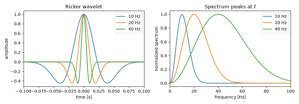
Norman Ricker studied how a sharp seismic pulse changes shape as it travels through absorbing rock and proposed the “Mexican hat” pulse as its stable form. The wavelet has unit peak, zero mean, zero crossings at ±1/(sqrt(2) pi f) and an amplitude spectrum that peaks at f.

import matplotlib.pyplot as plt
import numpy as np

from earthsciencekit.seismology import ricker_wavelet

dt = 1e-4
time = np.arange(-0.5, 0.5, dt)
fig, axes = plt.subplots(1, 2, figsize=(10, 3.5))
for f in [10, 20, 40]:
    pulse = ricker_wavelet(time, f)
    assert np.isclose(ricker_wavelet(1 / (np.sqrt(2) * np.pi * f), f), 0, atol=1e-15)
    assert abs(pulse.sum() * dt) < 1e-10
    spectrum = np.abs(np.fft.rfft(pulse))
    freq = np.fft.rfftfreq(time.size, dt)
    assert abs(freq[np.argmax(spectrum)] - f) <= freq[1]
    axes[0].plot(time, pulse, label=f"{f} Hz")
    axes[1].plot(freq, spectrum / spectrum.max(), label=f"{f} Hz")
axes[0].set(xlim=(-0.1, 0.1), xlabel="time [s]", ylabel="amplitude", title="Ricker wavelet")
axes[1].set(xlim=(0, 100), xlabel="frequency [Hz]", ylabel="normalized spectrum", title="Spectrum peaks at f")
for ax in axes:
    ax.legend()
fig.tight_layout()

plt.show()