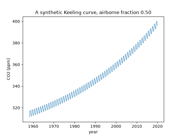
Keeling’s curve (1958)

Charles David Keeling began continuous measurements of carbon dioxide at Mauna Loa in 1958. Within two years the record showed a seasonal cycle from the breathing of northern forests and a steady rise. Here the rise is synthetic: emissions grow by 2% a year and each pulse decays in a single reservoir with a 50-year time scale. For steady exponential growth, the fraction of emitted carbon left in the air tends to g tau / (1 + g tau), here one half.

import matplotlib.pyplot as plt
import numpy as np

from earthsciencekit.climate import carbon_airborne_fraction, carbon_decay
from earthsciencekit.units import convert

growth, tau = 0.02, 50.0  # per year, years
years = np.arange(1750, 2020, 1 / 12)
dt = 1 / 12
emissions = 10e12 * np.exp(growth * (years - 2020))  # kg C per year
age = years[:, None] - years[None, :]
weight = carbon_decay(emissions[None, :] * dt, convert(tau, "year", "s"), convert(np.clip(age, 0, None), "year", "s"))
excess = np.where(age >= 0, weight, 0).sum(axis=1)
exact = 10e12 * (np.exp(growth * (years - 2020)) - np.exp(growth * (1750 - 2020) - (years - 1750) / tau)) / (growth + 1 / tau)
np.testing.assert_allclose(excess[120:], exact[120:], rtol=0.02)
fraction = carbon_airborne_fraction(excess[-1], emissions.sum() * dt)
assert np.isclose(fraction, growth * tau / (1 + growth * tau), atol=0.02)

ppm = 280 + excess / 2.12e12 + 3 * np.sin(2 * np.pi * (years - 0.3))
record = years >= 1958
fig, ax = plt.subplots()
ax.plot(years[record], ppm[record], lw=0.8)
ax.set(xlabel="year", ylabel="CO2 [ppm]", title=f"A synthetic Keeling curve, airborne fraction {fraction:.2f}")

plt.show()