Reid’s elastic rebound (1910)

From survey lines across the San Andreas fault before and after 1906, Harry Fielding Reid argued that the crust bends elastically while the fault is locked and springs back when it slips. Here a fault locked for 100 years stores the far-field motion as strain. At failure the stored offset is released in seconds, modelled as a damped oscillator returning to equilibrium.

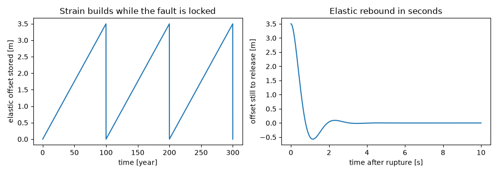
slip released per event: 3.50 m

import matplotlib.pyplot as plt
import numpy as np

from earthsciencekit.seismology import simulate_oscillator
from earthsciencekit.units import convert

rate = convert(3.5, "cm/year", "m/s")
recurrence = convert(100, "year", "s")
years = np.linspace(0, 300, 3001)
loading = convert(years, "year", "s")
slip_deficit = rate * np.mod(loading, recurrence)
stored = rate * recurrence
print(f"slip released per event: {stored:.2f} m")

# Coseismic rebound: the stored offset relaxes about the new equilibrium.
time = np.linspace(0, 10, 1001)
rebound = simulate_oscillator(0.5, 1.0, time, displacement=stored)
assert abs(rebound.values[-1, 0]) < 1e-3 * stored
assert np.isclose(rebound.values[0, 0], stored)

fig, axes = plt.subplots(1, 2, figsize=(10, 3.5))
axes[0].plot(years, slip_deficit)
axes[0].set(xlabel="time [year]", ylabel="elastic offset stored [m]", title="Strain builds while the fault is locked")
axes[1].plot(time, rebound.values[:, 0])
axes[1].set(xlabel="time after rupture [s]", ylabel="offset still to release [m]", title="Elastic rebound in seconds")
fig.tight_layout()

plt.show()