Callendar’s measured warming (1938)

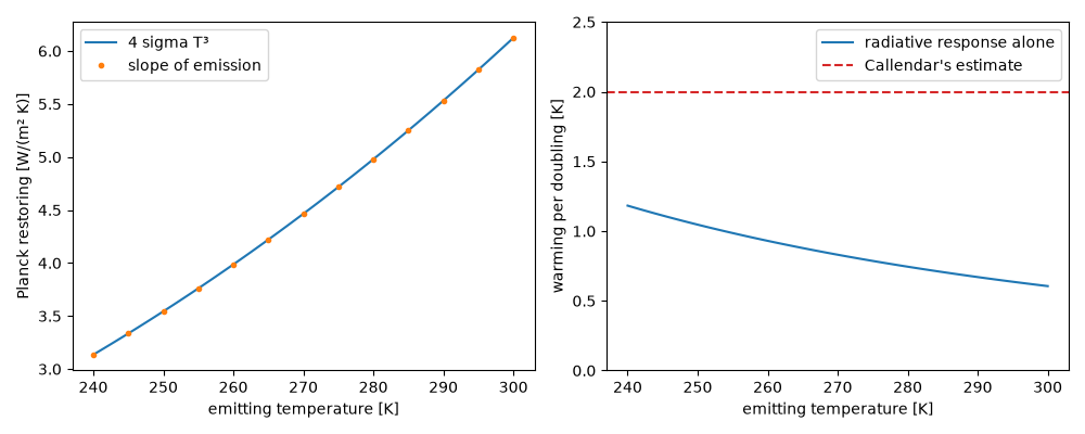
Guy Stewart Callendar compiled temperature records from about 200 stations, found that the world had warmed since the late 19th century, and attributed the warming to carbon dioxide from burning fuel. His estimate of about 2 °C per doubling was larger than the radiative response alone. Planck’s restoring coefficient 4 sigma T**3 gives only about 1 K per doubling, so feedbacks such as water vapour must amplify it.

import matplotlib.pyplot as plt
import numpy as np

from earthsciencekit.climate import co2_forcing, equilibrium_warming, outgoing_longwave, planck_feedback

temperature = np.linspace(240, 300, 121)
step = 0.01
numerical = (outgoing_longwave(temperature + step, 1) - outgoing_longwave(temperature - step, 1)) / (2 * step)
np.testing.assert_allclose(numerical, planck_feedback(temperature, 1), rtol=1e-8)
doubling = co2_forcing(560, 280, 5.35)
planck_only = equilibrium_warming(doubling, planck_feedback(temperature, 1))
assert 0.9 < equilibrium_warming(doubling, planck_feedback(255, 1)) < 1.1

fig, (left, right) = plt.subplots(1, 2, figsize=(10, 4))
left.plot(temperature, planck_feedback(temperature, 1), label="4 sigma T³")
left.plot(temperature[::10], numerical[::10], ".", label="slope of emission")
left.set(xlabel="emitting temperature [K]", ylabel="Planck restoring [W/(m² K)]")
left.legend()
right.plot(temperature, planck_only, label="radiative response alone")
right.axhline(2.0, color="tab:red", ls="--", label="Callendar's estimate")
right.set(xlabel="emitting temperature [K]", ylabel="warming per doubling [K]", ylim=(0, 2.5))
right.legend()
fig.tight_layout()

plt.show()