Theis’s well solution (1935)

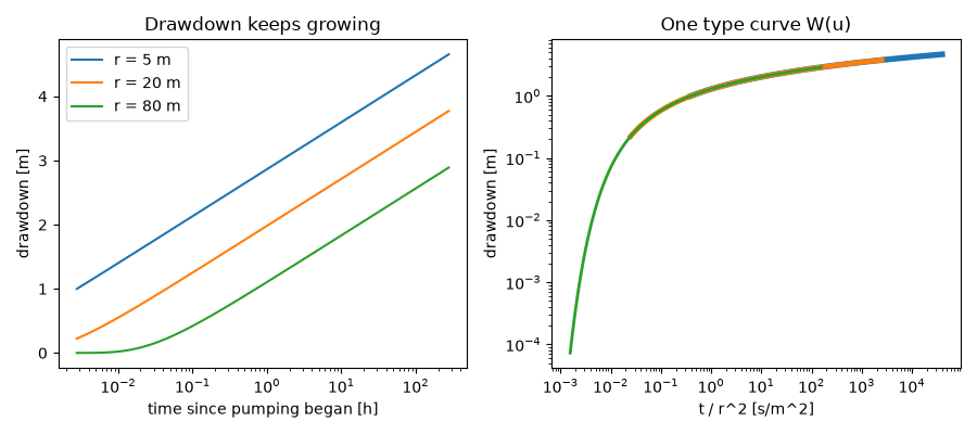
Charles Theis noticed that groundwater flow to a well obeys the same equation as heat conduction, and borrowed the solution for a line sink. The drawdown grows without limit as the well takes water from storage, at a rate fixed by the transmissivity, and every observation well falls on one type curve when the drawdown is plotted against t / r**2.

import matplotlib.pyplot as plt
import numpy as np

from earthsciencekit.hydrology import theis_drawdown, well_function

rate, transmissivity, storativity = 0.02, 5e-3, 2e-4
time = np.logspace(1, 6, 200)
fig, (left, right) = plt.subplots(1, 2, figsize=(9, 4))
for radius in (5.0, 20.0, 80.0):
    drawdown = theis_drawdown(rate, transmissivity, storativity, radius, time)
    u = radius**2 * storativity / (4 * transmissivity * time)
    assert np.allclose(drawdown, rate / (4 * np.pi * transmissivity) * well_function(u))
    left.semilogx(time / 3600, drawdown, label=f"r = {radius:g} m")
    right.loglog(time / radius**2, drawdown, lw=4 - radius / 40, label=f"r = {radius:g} m")
left.set(xlabel="time since pumping began [h]", ylabel="drawdown [m]", title="Drawdown keeps growing")
right.set(xlabel="t / r^2 [s/m^2]", ylabel="drawdown [m]", title="One type curve W(u)")
left.legend()
fig.tight_layout()

plt.show()