Libby’s radiocarbon dating (1949)

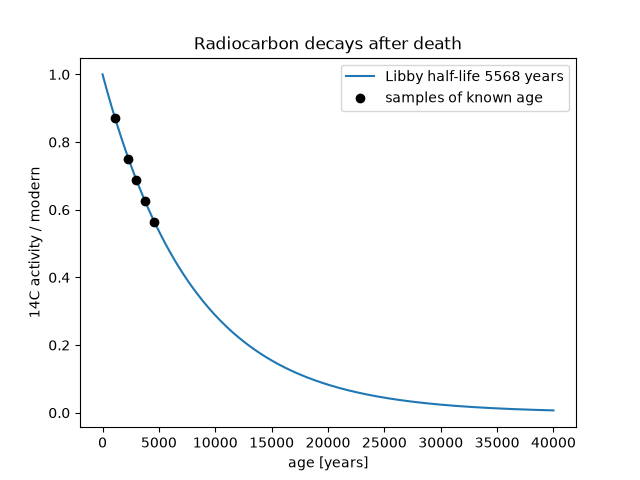
Willard Libby reasoned that cosmic rays keep the atmosphere’s carbon-14 in a steady state, that living things share it, and that it decays once they die. Arnold and Libby tested the idea on wood and grain of known historical age and found their “curve of knowns”. Conventional ages still use Libby’s 5568-year half-life; the better value of 5730 years makes true ages about 3% older.

import matplotlib.pyplot as plt
import numpy as np

from earthsciencekit.units import convert
from earthsciencekit.volcanology import decay_constant, parent_fraction, radiocarbon_age

known = convert(np.array([1100, 2300, 3000, 3750, 4600]), "year", "s")  # synthetic samples of known age
fraction = parent_fraction(decay_constant(convert(5568, "year", "s")), known)
assert np.allclose(radiocarbon_age(fraction), known, rtol=1e-4)
cambridge = parent_fraction(decay_constant(convert(5730, "year", "s")), known)
assert np.allclose(radiocarbon_age(cambridge) / known, 5568 / 5730, rtol=1e-4)

age = convert(np.linspace(0, 40000, 400), "year", "s")
fig, ax = plt.subplots()
ax.plot(convert(age, "s", "year"), parent_fraction(decay_constant(convert(5568, "year", "s")), age), label="Libby half-life 5568 years")
ax.plot(convert(known, "s", "year"), fraction, "ko", label="samples of known age")
ax.set(xlabel="age [years]", ylabel="14C activity / modern", title="Radiocarbon decays after death")
ax.legend()

plt.show()