TEOS-10 (2010)

The Thermodynamic Equation of Seawater 2010 replaced the 1980 equation of state with one derived from a Gibbs function, in Absolute Salinity and Conservative Temperature. Its density is curved in temperature: mixing two waters of equal density gives a denser mixture (cabbeling), which no linear equation of state can show. Here the simplified fit of Roquet et al. (2015) stands in for the full TEOS-10 polynomial.

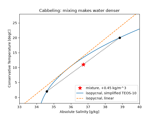
mixing two waters of 1026.69 kg/m^3 gives 1027.14 kg/m^3

import matplotlib.pyplot as plt
import numpy as np
from scipy.optimize import brentq

from earthsciencekit.oceanography import linear_density, simplified_seawater_density
from earthsciencekit.units import convert

alpha, beta = 0.16550 / 1026, 0.76554 / 1026
cold = (convert(2.0, "degC", "K"), 34.6)
target = simplified_seawater_density(*cold, 0)
warm_salinity = brentq(lambda s: simplified_seawater_density(convert(20.0, "degC", "K"), s, 0) - target, 30, 45, xtol=1e-14)
warm = (convert(20.0, "degC", "K"), warm_salinity)
mixed = simplified_seawater_density((cold[0] + warm[0]) / 2, (cold[1] + warm[1]) / 2, 0)
assert mixed > target + 0.1
linear_cold = linear_density(1026, cold[0] - 283.15, cold[1] - 35, alpha, beta)
linear_warm = linear_density(1026, warm[0] - 283.15, warm[1] - 35, alpha, beta)
linear_mix = linear_density(1026, (cold[0] + warm[0]) / 2 - 283.15, (cold[1] + warm[1]) / 2 - 35, alpha, beta)
assert np.isclose(linear_mix, (linear_cold + linear_warm) / 2)
print(f"mixing two waters of {target:.2f} kg/m^3 gives {mixed:.2f} kg/m^3")

salinity, celsius = np.meshgrid(np.linspace(33, 40, 141), np.linspace(-2, 28, 121))
kelvin = convert(celsius, "degC", "K")
fig, ax = plt.subplots()
ax.contour(salinity, celsius, simplified_seawater_density(kelvin, salinity, 0), levels=[target], colors="tab:blue")
ax.contour(
    salinity,
    celsius,
    linear_density(1026, kelvin - 283.15, salinity - 35, alpha, beta),
    levels=[target],
    colors="tab:orange",
    linestyles="--",
)
ax.plot([cold[1], warm[1]], [2, 20], "k:o")
ax.plot((cold[1] + warm[1]) / 2, 11, "r*", markersize=12, label=f"mixture, +{mixed - target:.2f} kg/m^3")
ax.plot([], [], color="tab:blue", label="isopycnal, simplified TEOS-10")
ax.plot([], [], color="tab:orange", ls="--", label="isopycnal, linear")
ax.set(xlabel="Absolute Salinity [g/kg]", ylabel="Conservative Temperature [degC]", title="Cabbeling: mixing makes water denser")
ax.legend(loc="lower right")

plt.show()