Bjerknes’s forecasting programme (1904)

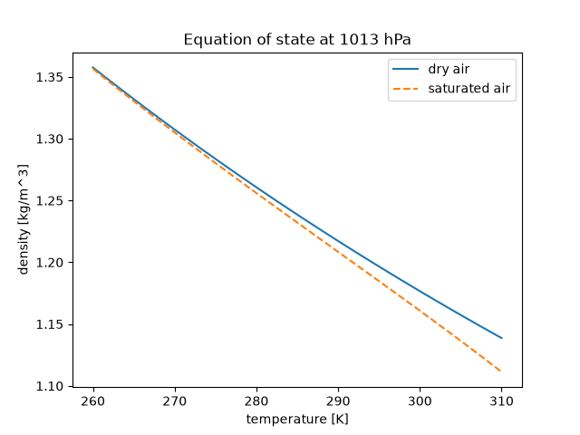
Vilhelm Bjerknes argued that weather forecasting is a problem of mechanics and physics: seven variables (pressure, density, temperature, humidity and three wind components) and seven equations. The equation of state is the diagnostic one that ties pressure, density and temperature together. Moist air obeys it with the virtual temperature in place of temperature, so it is lighter than dry air at the same pressure and temperature. The check is that the result equals the sum of Dalton’s partial densities.

import matplotlib.pyplot as plt
import numpy as np

from earthsciencekit.atmosphere import dry_air_density, mixing_ratio, saturation_vapor_pressure, specific_humidity, virtual_temperature
from earthsciencekit.constants import R_DRY_AIR, R_VAPOR

pressure = 101325.0
temperature = np.linspace(260, 310, 101)
vapor = saturation_vapor_pressure(temperature)
q = specific_humidity(mixing_ratio(vapor, pressure))
moist = dry_air_density(pressure, virtual_temperature(temperature, q))
dry = dry_air_density(pressure, temperature)
np.testing.assert_allclose(moist, (pressure - vapor) / (R_DRY_AIR * temperature) + vapor / (R_VAPOR * temperature))
assert np.all(moist < dry)

fig, ax = plt.subplots()
ax.plot(temperature, dry, label="dry air")
ax.plot(temperature, moist, ls="--", label="saturated air")
ax.set(xlabel="temperature [K]", ylabel="density [kg/m^3]", title=f"Equation of state at {pressure / 100:.0f} hPa")
ax.legend()

plt.show()