Laplace’s tidal equations (1776)

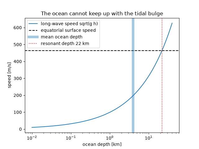
Pierre-Simon Laplace replaced Newton’s static bulge with the dynamics of a thin ocean on a rotating Earth. Long waves in that ocean travel at sqrt(g h). To keep pace with the Moon’s bulge at the equator the ocean would have to be about 22 km deep; the real ocean, about 4 km deep, cannot follow it, so real tides are a forced dynamic response, not an equilibrium.

import matplotlib.pyplot as plt
import numpy as np

from earthsciencekit.constants import EARTH_RADIUS, GRAVITY, OMEGA_EARTH
from earthsciencekit.oceanography import shallow_wave_speed

surface_speed = OMEGA_EARTH * EARTH_RADIUS
critical_depth = surface_speed**2 / GRAVITY
assert np.isclose(shallow_wave_speed(critical_depth, GRAVITY), surface_speed)
assert 21e3 < critical_depth < 23e3
assert shallow_wave_speed(4000, GRAVITY) < 0.5 * surface_speed

depth = np.logspace(1, np.log10(40e3), 300)
fig, ax = plt.subplots()
ax.semilogx(depth / 1e3, shallow_wave_speed(depth, GRAVITY), label="long-wave speed sqrt(g h)")
ax.axhline(surface_speed, color="k", ls="--", label="equatorial surface speed")
ax.axvline(4, color="tab:blue", alpha=0.4, lw=6, label="mean ocean depth")
ax.axvline(critical_depth / 1e3, color="tab:red", ls=":", label=f"resonant depth {critical_depth / 1e3:.0f} km")
ax.set(xlabel="ocean depth [km]", ylabel="speed [m/s]", title="The ocean cannot keep up with the tidal bulge")
ax.legend()

plt.show()