Hertz’s floating elastic plate (1884)

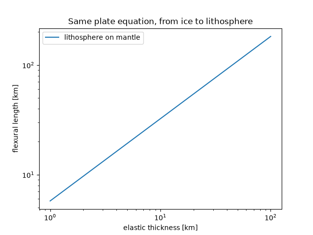
Heinrich Hertz solved for the bending of a thin elastic plate floating on a fluid, the problem of a load on lake ice. The same equation describes the lithosphere floating on the mantle: rigidity grows as the cube of the elastic thickness and the flexural length as its three-quarter power.

flexural length of 0.5 m lake ice: 14.4 m
flexural length of a 30 km plate: 74 km

import matplotlib.pyplot as plt
import numpy as np

from earthsciencekit.constants import GRAVITY
from earthsciencekit.plate_tectonics import flexural_parameter, flexural_rigidity

ice = flexural_parameter(flexural_rigidity(9e9, 0.5, 0.33), 1000, GRAVITY)
thickness = np.logspace(3, 5, 50)
rigidity = flexural_rigidity(7e10, thickness, 0.25)
alpha = flexural_parameter(rigidity, 3300 - 1000, GRAVITY)
assert np.isclose(np.polyfit(np.log(thickness), np.log(alpha), 1)[0], 0.75)
assert np.isclose(np.polyfit(np.log(thickness), np.log(rigidity), 1)[0], 3)
print(f"flexural length of 0.5 m lake ice: {float(ice):.1f} m")
print(f"flexural length of a 30 km plate: {float(flexural_parameter(flexural_rigidity(7e10, 30e3, 0.25), 2300, GRAVITY)) / 1e3:.0f} km")

fig, ax = plt.subplots()
ax.loglog(thickness / 1e3, alpha / 1e3, label="lithosphere on mantle")
ax.set(xlabel="elastic thickness [km]", ylabel="flexural length [km]", title="Same plate equation, from ice to lithosphere")
ax.legend()

plt.show()