Stefan’s sea-ice growth (1891)

Josef Stefan treated the growth of polar sea ice as a moving-boundary problem: the latent heat released as water freezes at the base must be conducted up through the ice already formed. The thickness then grows as the square root of the freezing degree-days, so four times the cold makes only twice the ice. The example integrates a synthetic Arctic winter.

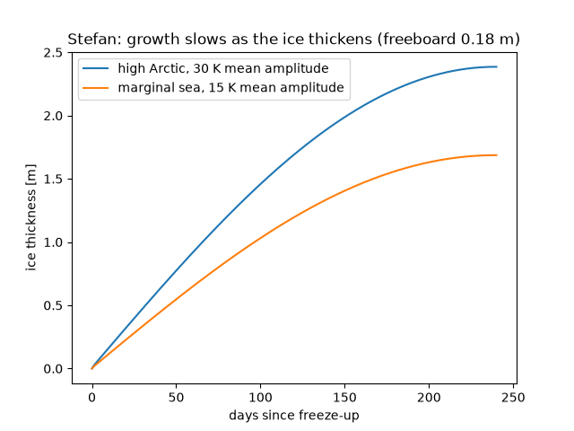
import matplotlib.pyplot as plt
import numpy as np

from earthsciencekit.constants import ICE_DENSITY, LATENT_HEAT_FUSION
from earthsciencekit.glaciology import sea_ice_freeboard, stefan_ice_thickness

conductivity, freezing = 2.2, 271.35  # W/(m K), K for seawater
day = np.arange(0, 241)
fig, ax = plt.subplots()
for amplitude, label in [(30, "high Arctic"), (15, "marginal sea")]:
    air = freezing - amplitude * np.sin(np.pi * day / 240)
    degree_seconds = np.concatenate([[0], np.cumsum(freezing - air[1:])]) * 86400
    thickness = stefan_ice_thickness(degree_seconds, conductivity, ICE_DENSITY, LATENT_HEAT_FUSION)
    ax.plot(day, thickness, label=f"{label}, {amplitude} K mean amplitude")
quadrupled = stefan_ice_thickness(4e8, conductivity, ICE_DENSITY, LATENT_HEAT_FUSION)
assert np.isclose(quadrupled, 2 * stefan_ice_thickness(1e8, conductivity, ICE_DENSITY, LATENT_HEAT_FUSION))
freeboard = sea_ice_freeboard(thickness[-1], ICE_DENSITY, 1025)
title = f"Stefan: growth slows as the ice thickens (freeboard {freeboard:.2f} m)"
ax.set(xlabel="days since freeze-up", ylabel="ice thickness [m]", title=title)
ax.legend()

plt.show()