Horton’s laws of stream numbers (1945)

Robert Horton ordered the streams of a basin, from unbranched headwaters up to the main river, and found that the number of streams of each order falls in a geometric series while their mean length grows in another. Two ratios, the bifurcation ratio and the length ratio, summarize the whole network. The example fits both to a synthetic fifth-order basin (with Strahler’s 1952 ordering) and compares the counts with Horton’s law.

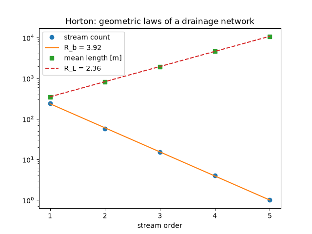
import matplotlib.pyplot as plt
import numpy as np

from earthsciencekit.hydrology import stream_length, stream_number

order = np.arange(1, 6)
counts = np.array([243, 58, 15, 4, 1])
lengths = np.array([0.35, 0.82, 1.9, 4.6, 10.8]) * 1e3  # m
bifurcation = 10 ** -np.polyfit(order, np.log10(counts), 1)[0]
length_ratio = 10 ** np.polyfit(order, np.log10(lengths), 1)[0]
predicted = stream_number(order, 5, bifurcation)
assert 3.5 < bifurcation < 4.5 and 2 < length_ratio < 2.6
assert np.all(np.abs(np.log(predicted / counts)) < 0.25)

fig, ax = plt.subplots()
ax.semilogy(order, counts, "o", label="stream count")
ax.semilogy(order, predicted, "-", label=f"R_b = {bifurcation:.2f}")
ax.semilogy(order, lengths, "s", label="mean length [m]")
ax.semilogy(order, stream_length(order, stream_length(1, lengths[0], 1), length_ratio), "--", label=f"R_L = {length_ratio:.2f}")
ax.set(xlabel="stream order", xticks=order, title="Horton: geometric laws of a drainage network")
ax.legend()

plt.show()