Omori’s aftershock decay (1894)

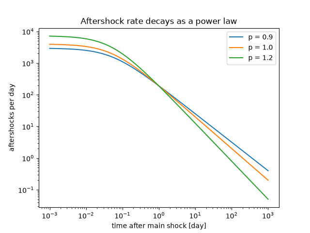
Fusakichi Omori counted the aftershocks of the 1891 Nobi earthquake and found that their rate fell as 1/(t + c). Tokuji Utsu later generalized the exponent to p, usually close to 1. On log-log axes the rate is flat for t << c and has slope -p for t >> c. The parameters here are synthetic.

import matplotlib.pyplot as plt
import numpy as np

from earthsciencekit.seismology import omori_rate
from earthsciencekit.units import convert

day = convert(1, "day", "s")
time = np.logspace(-3, 3, 300) * day
c, k = 0.05 * day, 200.0
fig, ax = plt.subplots()
for p in [0.9, 1.0, 1.2]:
    rate = omori_rate(k * day ** (p - 1), c, p, time) * day
    ax.loglog(time / day, rate, label=f"p = {p}")
    late = time > 100 * c
    slope = np.polyfit(np.log(time[late] + c), np.log(rate[late]), 1)[0]
    assert np.isclose(slope, -p)

# Omori's original law integrates to a logarithm: N(T) = K ln(1 + T / c).
t = np.linspace(0, 30 * day, 30001)
count = np.trapezoid(omori_rate(k, c, 1.0, t), t)
assert np.isclose(count, k * np.log1p(30 * day / c), rtol=1e-4)
ax.set(xlabel="time after main shock [day]", ylabel="aftershocks per day", title="Aftershock rate decays as a power law")
ax.legend()

plt.show()