Green and Ampt’s infiltration (1911)

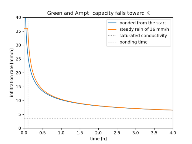
W. Heber Green and G. A. Ampt pictured water entering a soil as a sharp wetting front, saturated above and dry below, pulled down by gravity and by the capillary suction at the front. The infiltration rate starts high, falls as the wetted zone deepens and tends to the saturated conductivity. Under steady rain the soil first absorbs everything; once its capacity falls to the rain rate the surface ponds and the excess runs off, as in Mein and Larson’s (1973) treatment, which simulate_infiltration integrates.

import matplotlib.pyplot as plt
import numpy as np

from earthsciencekit.hydrology import green_ampt_rate, green_ampt_time, simulate_infiltration

conductivity, suction, deficit = 1e-6, 0.11, 0.3  # a loam
depth = np.linspace(1e-4, 0.08, 400)
ponded_time = green_ampt_time(depth, conductivity, suction, deficit)
time = np.linspace(0, 4 * 3600, 481)
storm = simulate_infiltration(conductivity, suction, deficit, 1e-5, time)
rate = storm.values[:, 1]
ponding = time[np.argmax(storm.values[:, 2] > 0)]
expected = conductivity * suction * deficit / (1e-5 * (1e-5 - conductivity))
assert abs(ponding - expected) <= time[1] and np.isclose(green_ampt_rate(1e3, conductivity, suction, deficit), conductivity, rtol=1e-4)

fig, ax = plt.subplots()
ax.plot(ponded_time / 3600, green_ampt_rate(depth, conductivity, suction, deficit) * 3.6e6, label="ponded from the start")
ax.plot(time / 3600, rate * 3.6e6, label="steady rain of 36 mm/h")
ax.axhline(conductivity * 3.6e6, color="0.5", ls=":", label="saturated conductivity")
ax.axvline(expected / 3600, color="0.7", ls="--", lw=1, label="ponding time")
ax.set(xlim=(0, 4), ylim=(0, 40), xlabel="time [h]", ylabel="infiltration rate [mm/h]", title="Green and Ampt: capacity falls toward K")
ax.legend()

plt.show()