Väisälä and Brunt’s buoyancy frequency (1925)

Vilho Väisälä (1925) and David Brunt (1927) showed that a parcel displaced vertically in stable air oscillates about its level, with angular frequency N = sqrt(g / theta * dtheta/dz). In the troposphere the period is about ten minutes. Integrating the parcel equation z'' = -N^2 z recovers that period.

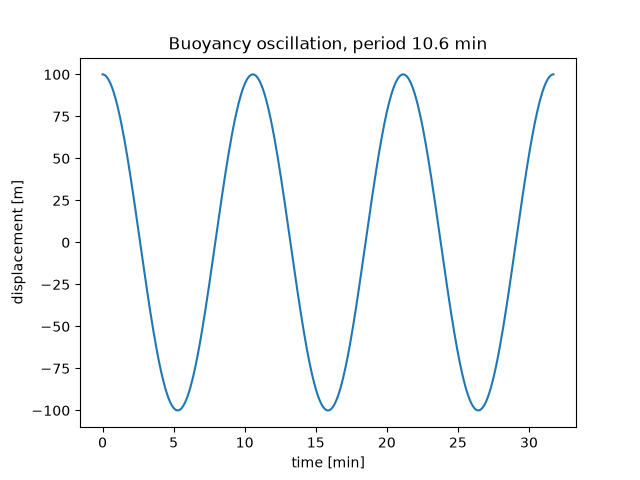
buoyancy period: 10.6 min

import matplotlib.pyplot as plt
import numpy as np

from earthsciencekit.atmosphere import brunt_vaisala_squared
from earthsciencekit.constants import GRAVITY
from earthsciencekit.integrators import integrate_ode

n2 = float(brunt_vaisala_squared(300, 0.003, GRAVITY))
period = 2 * np.pi / np.sqrt(n2)
time = np.linspace(0, 3 * period, 601)
result = integrate_ode(lambda t, y: [y[1], -n2 * y[0]], [100.0, 0.0], time, names=("height", "speed"), units=("m", "m/s"))
np.testing.assert_allclose(result.values[:, 0], 100 * np.cos(np.sqrt(n2) * time), atol=1e-4)
print(f"buoyancy period: {period / 60:.1f} min")

fig, ax = plt.subplots()
ax.plot(time / 60, result.values[:, 0])
ax.set(xlabel="time [min]", ylabel="displacement [m]", title=f"Buoyancy oscillation, period {period / 60:.1f} min")

plt.show()