Sandström and Helland-Hansen’s dynamic method (1903)

Johan Sandström and Bjørn Helland-Hansen showed how to compute currents from temperature and salinity alone. Light water stands higher than dense water, so the sea surface above a warm station rises relative to a cold one until the pressure at a deep level of no motion is the same under both. The surface slope then drives a geostrophic current.

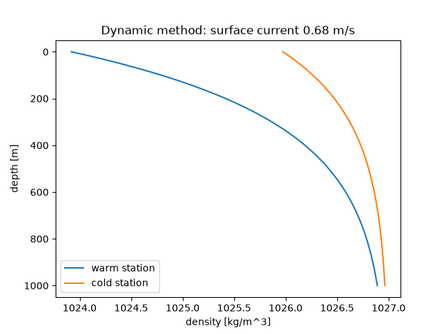
surface height difference 58 cm, current 0.68 m/s

import matplotlib.pyplot as plt
import numpy as np

from earthsciencekit.atmosphere import coriolis_parameter
from earthsciencekit.constants import GRAVITY
from earthsciencekit.oceanography import geostrophic_current, hydrostatic_pressure, linear_density

reference, distance = 1027.0, 100e3
depth = np.linspace(0, 1000, 2001)
stations = {"warm": 15 * np.exp(-depth / 300), "cold": 5 * np.exp(-depth / 300)}
density = {name: linear_density(reference, anomaly, 0, 2e-4, 7.6e-4) for name, anomaly in stations.items()}
height = {name: np.trapezoid(reference - rho, depth) / reference for name, rho in density.items()}
bottom = {
    name: hydrostatic_pressure(reference, height[name], GRAVITY) + GRAVITY * np.trapezoid(rho, depth) for name, rho in density.items()
}
assert np.isclose(bottom["warm"], bottom["cold"])

slope = (height["warm"] - height["cold"]) / distance
speed = geostrophic_current(slope, coriolis_parameter(np.radians(35)), GRAVITY)
assert 0.3 < speed < 2
print(f"surface height difference {100 * (height['warm'] - height['cold']):.0f} cm, current {speed:.2f} m/s")

fig, ax = plt.subplots()
for name, rho in density.items():
    ax.plot(rho, depth, label=f"{name} station")
ax.invert_yaxis()
ax.set(xlabel="density [kg/m^3]", ylabel="depth [m]", title=f"Dynamic method: surface current {speed:.2f} m/s")
ax.legend()

plt.show()