Mohorovičić’s discontinuity (1909)

On records of the Kupa Valley earthquake of 8 October 1909, Andrija Mohorovičić saw two P phases. A few hundred kilometres out a faster phase overtook the direct wave: energy refracted along a boundary below the crust. The crossover distance fixes the depth of that boundary, which he put at about 54 km. The speeds below are of the size he used.

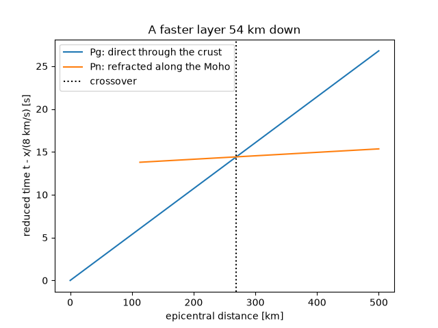
crossover at 269 km; head wave starts at 113 km

import matplotlib.pyplot as plt
import numpy as np

from earthsciencekit.seismology import critical_angle, crossover_distance, head_wave_travel_time, travel_time

h, v_crust, v_mantle = 54e3, 5.6e3, 7.75e3
x_cross = crossover_distance(h, v_crust, v_mantle)
x_crit = 2 * h * np.tan(critical_angle(v_crust, v_mantle))
assert np.isclose(head_wave_travel_time(x_cross, h, v_crust, v_mantle), travel_time(x_cross, v_crust))
print(f"crossover at {x_cross / 1e3:.0f} km; head wave starts at {x_crit / 1e3:.0f} km")

x = np.linspace(0, 500e3, 501)
x_head = x[x >= x_crit]
fig, ax = plt.subplots()
ax.plot(x / 1e3, travel_time(x, v_crust) - x / 8e3, label="Pg: direct through the crust")
ax.plot(x_head / 1e3, head_wave_travel_time(x_head, h, v_crust, v_mantle) - x_head / 8e3, label="Pn: refracted along the Moho")
ax.axvline(x_cross / 1e3, color="k", ls=":", label="crossover")
ax.set(xlabel="epicentral distance [km]", ylabel="reduced time t - x/(8 km/s) [s]", title="A faster layer 54 km down")
ax.legend()

plt.show()