Myhre’s forcing formulas (1998)

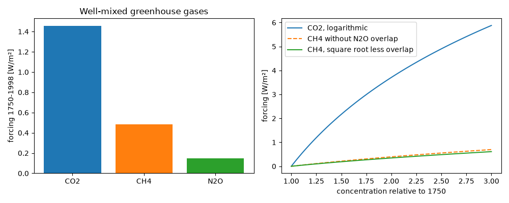
Gunnar Myhre and colleagues fitted simple expressions to line-by-line radiative calculations for the well-mixed greenhouse gases. CO2 forcing is logarithmic, 5.35 ln(C / C0), because its strongest bands are saturated. Methane and nitrous oxide grow with the square root of concentration, less a term for the band near 7.7 μm that they share. The IPCC adopted the formulas in 2001; from 1750 to 1998 they give about 1.46, 0.48 and 0.15 W/m² for the three gases.

import matplotlib.pyplot as plt
import numpy as np

from earthsciencekit.climate import co2_forcing, methane_forcing, nitrous_oxide_forcing

values = {
    "CO2": co2_forcing(365, 278, 5.35),
    "CH4": methane_forcing(1745, 700, 270),
    "N2O": nitrous_oxide_forcing(314, 270, 700),
}
np.testing.assert_allclose(list(values.values()), [1.46, 0.48, 0.15], atol=0.01)
ratio = np.linspace(1, 3, 101)
overlap_free = methane_forcing(700 * ratio, 700, 1e-6)
with_overlap = methane_forcing(700 * ratio, 700, 270)
assert np.all(with_overlap[1:] < overlap_free[1:])

fig, (left, right) = plt.subplots(1, 2, figsize=(10, 4))
left.bar(list(values), list(values.values()), color=["C0", "C1", "C2"])
left.set(ylabel="forcing 1750-1998 [W/m²]", title="Well-mixed greenhouse gases")
right.plot(ratio, co2_forcing(278 * ratio, 278, 5.35), label="CO2, logarithmic")
right.plot(ratio, overlap_free, "--", label="CH4 without N2O overlap")
right.plot(ratio, with_overlap, label="CH4, square root less overlap")
right.set(xlabel="concentration relative to 1750", ylabel="forcing [W/m²]")
right.legend()
fig.tight_layout()

plt.show()