Schoof’s grounding-line flux (2007)

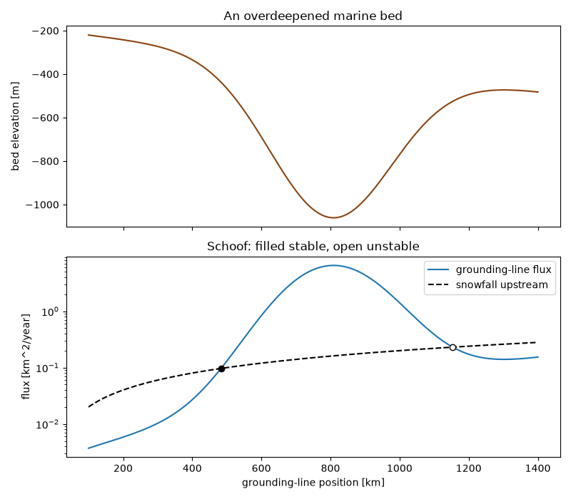
Christian Schoof resolved the boundary layer where a sliding ice sheet meets its shelf and found that the flux across the grounding line is a power of the flotation thickness, about 4.75 for Glen’s n = 3 and a sliding exponent of 1/3. A grounding line is steady where this flux equals the snowfall upstream, and stable only where the bed rises inland. On an overdeepened bed the steady states come in pairs, and the inner one is unstable.

import matplotlib.pyplot as plt
import numpy as np

from earthsciencekit.constants import GRAVITY, ICE_DENSITY, SECONDS_PER_YEAR
from earthsciencekit.glaciology import flotation_thickness, schoof_grounding_line_flux

parameters = (2.4e-25, 3, 7.6e6, 1 / 3, ICE_DENSITY, 1028, GRAVITY)
x = np.linspace(100e3, 1400e3, 1301)
bed_depth = 200 + 700 * np.exp(-(((x - 800e3) / 250e3) ** 2)) + 2e-4 * x  # an overdeepening
flux = schoof_grounding_line_flux(flotation_thickness(bed_depth, ICE_DENSITY, 1028), *parameters)
supply = 0.2 / SECONDS_PER_YEAR * x
ratio = schoof_grounding_line_flux(2000, *parameters) / schoof_grounding_line_flux(1000, *parameters)
assert np.isclose(ratio, 2**4.75)
imbalance = flux - supply
crossings = np.flatnonzero(np.diff(np.sign(imbalance)))
stable = np.gradient(imbalance, x)[crossings] > 0
assert crossings.size >= 2 and stable.any() and not stable.all()

fig, (top, bottom) = plt.subplots(2, 1, figsize=(8, 7), sharex=True)
top.plot(x / 1e3, -bed_depth, color="saddlebrown")
top.set(ylabel="bed elevation [m]", title="An overdeepened marine bed")
bottom.semilogy(x / 1e3, flux * SECONDS_PER_YEAR / 1e6, label="grounding-line flux")
bottom.semilogy(x / 1e3, supply * SECONDS_PER_YEAR / 1e6, "k--", label="snowfall upstream")
for index, ok in zip(crossings, stable):
    bottom.plot(x[index] / 1e3, supply[index] * SECONDS_PER_YEAR / 1e6, "o", color="k", mfc="k" if ok else "white")
bottom.set(xlabel="grounding-line position [km]", ylabel="flux [km^2/year]", title="Schoof: filled stable, open unstable")
bottom.legend()
fig.tight_layout()

plt.show()