Cox, Doell and Dalrymple’s polarity timescale (1964)

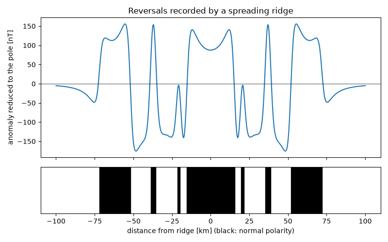
Allan Cox, Richard Doell and Brent Dalrymple dated lava flows from around the world by potassium-argon and measured their polarity. Flows of the same age had the same polarity everywhere, so reversals are global and can be put on a clock: the Brunhes normal epoch, the reversed Matuyama with short normal events, and the normal Gauss. The timescale turned the magnetic stripes at ridges into a speedometer. Spreading crust records it as blocks of alternating magnetization, whose anomaly profile is symmetric about the ridge.

import matplotlib.pyplot as plt
import numpy as np

from earthsciencekit.geophysics import block_magnetic_anomaly
from earthsciencekit.units import convert

normal_chrons = [(0.0, 0.773), (0.988, 1.072), (1.775, 1.934), (2.595, 3.596)]  # Ma
boundaries = sorted({0.0, 3.596, *(t for chron in normal_chrons for t in chron)})
rate = convert(2.0, "cm/year", "m/s")  # half spreading rate
x = np.linspace(-1e5, 1e5, 801)
anomaly = np.zeros_like(x)
for start, end in zip(boundaries[:-1], boundaries[1:]):
    sign = 1 if any(lo <= start < hi for lo, hi in normal_chrons) else -1
    near, far = rate * convert(start, "Ma", "s"), rate * convert(end, "Ma", "s")
    for left, right in [(near, far), (-far, -near)]:
        anomaly += block_magnetic_anomaly(x, left, right, 3000, 3500, sign * 5)
anomaly = convert(anomaly, "T", "nT")
np.testing.assert_allclose(anomaly, anomaly[::-1], atol=1e-9)
matuyama = np.abs(x - rate * convert(1.4, "Ma", "s")).argmin()
assert anomaly[x.size // 2] > 0 > anomaly[matuyama]

fig, (top, bottom) = plt.subplots(2, 1, sharex=True, figsize=(8, 5), gridspec_kw={"height_ratios": [3, 1]})
top.plot(x / 1e3, anomaly)
top.axhline(0, color="k", lw=0.5)
top.set(ylabel="anomaly reduced to the pole [nT]", title="Reversals recorded by a spreading ridge")
for start, end in normal_chrons:
    for side in (1, -1):
        span = sorted([side * rate * convert(start, "Ma", "s") / 1e3, side * rate * convert(end, "Ma", "s") / 1e3])
        bottom.axvspan(*span, color="k")
bottom.set(xlabel="distance from ridge [km] (black: normal polarity)", yticks=[])
fig.tight_layout()

plt.show()