Haskell’s mantle viscosity from rebound (1935)

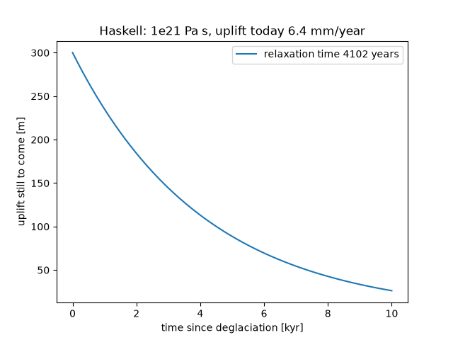
Norman Haskell treated the mantle under Fennoscandia as a viscous half-space and asked how fast a depression the size of the former ice sheet would recover. Matching the raised shorelines gave a viscosity of about 1e21 Pa s, still the standard value. The example builds a synthetic uplift history for a 3000 km depression and recovers the viscosity from the slope of its logarithm.

import matplotlib.pyplot as plt
import numpy as np

from earthsciencekit.constants import GRAVITY, SECONDS_PER_YEAR
from earthsciencekit.glaciology import haskell_viscosity, rebound_uplift_rate, remaining_depression, viscous_relaxation_time

wavelength, density = 3.0e6, 3300.0
tau = viscous_relaxation_time(wavelength, 1e21, density, GRAVITY)
time = np.linspace(0, 10e3, 201) * SECONDS_PER_YEAR
remaining = remaining_depression(time, 300.0, tau)
slope = np.polyfit(time, np.log(remaining), 1)[0]
assert np.isclose(haskell_viscosity(-1 / slope, wavelength, density, GRAVITY), 1e21)
rate_today = rebound_uplift_rate(time[-1], 300.0, tau) * SECONDS_PER_YEAR * 1e3

fig, ax = plt.subplots()
ax.plot(time / SECONDS_PER_YEAR / 1e3, remaining, label=f"relaxation time {tau / SECONDS_PER_YEAR:.0f} years")
title = f"Haskell: 1e21 Pa s, uplift today {rate_today:.1f} mm/year"
ax.set(xlabel="time since deglaciation [kyr]", ylabel="uplift still to come [m]", title=title)
ax.legend()

plt.show()