Charney, Fjørtoft and von Neumann’s ENIAC forecast (1950)

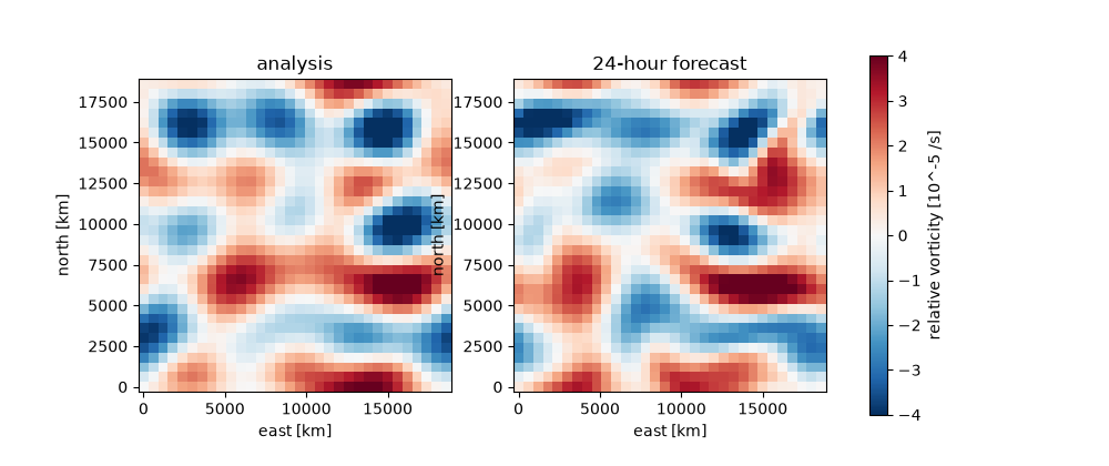
Jule Charney, Ragnar Fjørtoft and John von Neumann ran the first computer weather forecasts on the ENIAC in 1950. They avoided Richardson’s failure by predicting only the vorticity of a nondivergent barotropic flow, which keeps the fast gravity waves out. Here the same equation runs on a doubly periodic beta plane. A single Fourier mode is an exact Rossby wave and moves at the speed of Rossby’s formula; a mix of modes evolves nonlinearly while keeping its enstrophy.

import matplotlib.pyplot as plt
import numpy as np

from earthsciencekit.atmosphere import rossby_wave_speed, simulate_barotropic_vorticity

n, spacing, beta = 32, 600e3, 1.6e-11
x = np.arange(n) * spacing
X, Y = np.meshgrid(x, x)
length = n * spacing
day = 86400.0
k = 2 * np.pi * 2 / length
single = simulate_barotropic_vorticity(1e-5 * np.sin(k * X), [0, day], beta, spacing)
shift = float(rossby_wave_speed(0, beta, k)) * day
np.testing.assert_allclose(single.values[-1], 1e-5 * np.sin(k * (X - shift)).ravel(), atol=1e-10)

rng = np.random.default_rng(1950)
modes = [(i, j) for i in range(4) for j in range(-3, 4)]
zeta = sum(4e-6 * rng.normal() * np.cos(2 * np.pi * (i * X + j * Y) / length + rng.uniform(0, 2 * np.pi)) for i, j in modes)
result = simulate_barotropic_vorticity(zeta, [0, day], beta, spacing)
enstrophy = np.sum(result.values**2, axis=1)
assert np.isclose(enstrophy[-1], enstrophy[0], rtol=1e-5)

fig, axes = plt.subplots(1, 2, figsize=(10, 4.2))
for ax, field, title in zip(axes, result.values, ["analysis", "24-hour forecast"]):
    image = ax.pcolormesh(X / 1e3, Y / 1e3, field.reshape(n, n) * 1e5, cmap="RdBu_r", vmin=-4, vmax=4)
    ax.set(xlabel="east [km]", ylabel="north [km]", title=title, aspect="equal")
fig.colorbar(image, ax=axes, label="relative vorticity [10^-5 /s]")

plt.show()