Hadley’s circulation (1735)

George Hadley explained the trade winds. Air heated at the equator rises and flows poleward aloft, and air returns towards the equator near the ground. The ground there moves eastward faster than at the latitude the air came from, so the returning air lags behind and blows from the east. Today the deflection is written with the Coriolis parameter f = 2 Omega sin(phi). A ring of air that leaves the equator at rest and keeps its angular momentum gains the westerly wind Omega a sin^2(phi) / cos(phi), whose growth with latitude is f + u tan(phi) / a.

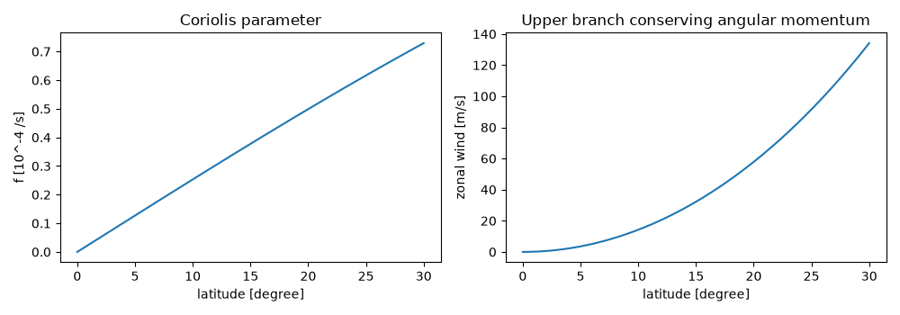
angular-momentum wind at 30 degrees: 134 m/s

import matplotlib.pyplot as plt
import numpy as np

from earthsciencekit.atmosphere import coriolis_parameter
from earthsciencekit.constants import EARTH_RADIUS, OMEGA_EARTH

latitude = np.deg2rad(np.linspace(0, 30, 301))
f = coriolis_parameter(latitude)
u = OMEGA_EARTH * EARTH_RADIUS * np.sin(latitude) ** 2 / np.cos(latitude)
dudy = np.gradient(u, EARTH_RADIUS * latitude)
np.testing.assert_allclose(dudy[1:-1], (f + u * np.tan(latitude) / EARTH_RADIUS)[1:-1], rtol=1e-3)
np.testing.assert_allclose(coriolis_parameter(-latitude), -f)
print(f"angular-momentum wind at 30 degrees: {u[-1]:.0f} m/s")

fig, axes = plt.subplots(1, 2, figsize=(10, 3.5))
axes[0].plot(np.rad2deg(latitude), f * 1e4)
axes[0].set(xlabel="latitude [degree]", ylabel="f [10^-4 /s]", title="Coriolis parameter")
axes[1].plot(np.rad2deg(latitude), u)
axes[1].set(xlabel="latitude [degree]", ylabel="zonal wind [m/s]", title="Upper branch conserving angular momentum")
fig.tight_layout()

plt.show()