Breakthroughs in Atmosphere#
Atmospheric science began with the discovery that air has weight. The
barometer of the 1640s led to hydrostatic balance and the logarithmic fall of
pressure with height, and the gas laws of the next two centuries added
adiabatic cooling, partial pressures and the saturation of water vapour.
Rotation entered with Hadley’s trade winds and Buys Ballot’s rule. After 1900,
balloon soundings revealed the stratosphere, and Bjerknes recast forecasting
as a problem in physics. Richardson’s failed hand forecast and the stability
and wave theories of the 1920s and 1930s prepared the barotropic vorticity
forecast that ran on the ENIAC in 1950. This chronology traces the results
behind earthsciencekit.atmosphere. Every example uses deterministic
synthetic inputs; none inverts real observations.
1643 – Torricelli’s Barometer#
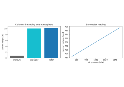
Evangelista Torricelli filled a glass tube with mercury and inverted it in a dish. The column fell to about 76 cm and left an empty space above it. He concluded that the weight of the surrounding air holds the column up: “we live submerged at the bottom of an ocean of the element air”. A water column would have to be 13.6 times taller, about 10 m.
Implementation: barometer_column_height()
(new).
References: E. Torricelli, letter to M. Ricci, 11 June 1644, in Opere di Evangelista Torricelli, vol. 3, ed. G. Loria and G. Vassura (Faenza, 1919): 186-188.
1648 – Pascal and Périer on the Puy de Dôme#
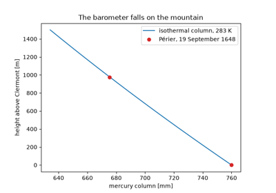
If the air’s weight holds up the mercury, the column should be shorter on a mountain. At Blaise Pascal’s request, Florin Périer carried a barometer up the Puy de Dôme on 19 September 1648. About 500 toises above Clermont, the column had fallen by 3 inches and 1.5 lines, while a control barometer in the town did not change. An isothermal hydrostatic column reproduces the drop to within a millimetre.
Implementation: barometric_pressure().
References: B. Pascal, Récit de la grande expérience de l’équilibre des liqueurs (Paris: Charles Savreux, 1648).
1686 – Halley’s Barometric Altitude#
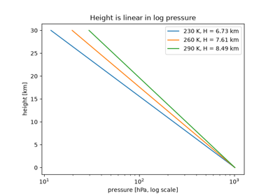
Edmond Halley combined Boyle’s law with the weight of the air and showed that
height above the ground grows with the logarithm of the pressure ratio. Equal
ratios of pressure mark equal steps of height, and the step for a factor e is
the scale height R T / g, about 8 km. The inverse of the barometric law is
the barometric altimeter.
Implementation: scale_height().
References: E. Halley, “A discourse of the rule of the decrease of the height of the mercury in the barometer, according as places are elevated above the surface of the earth,” Philosophical Transactions of the Royal Society of London 16 (1686): 104-116.
1735 – Hadley’s Circulation#
George Hadley explained the trade winds. Air heated near the equator rises and
flows poleward aloft, and surface air flows back towards the equator. The
Earth’s surface moves eastward faster near the equator than at the latitude
the returning air came from, so that air lags behind and blows from the east.
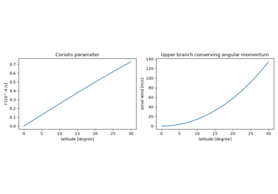
The modern form of the deflection is the Coriolis parameter
f = 2 Omega sin(phi).
Implementation: coriolis_parameter(). The
example checks that a ring of air conserving its angular momentum gains
westerly wind at the rate f + u tan(phi) / a.
References: G. Hadley, “Concerning the cause of the general trade-winds,” Philosophical Transactions of the Royal Society of London 39 (1735): 58-62.
1802 – Dalton’s Partial Pressures#
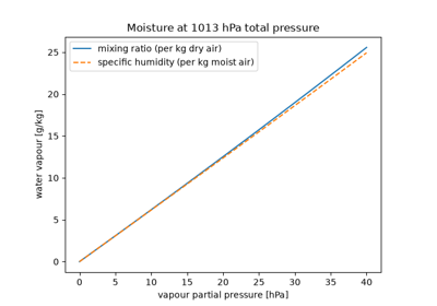
John Dalton found that each gas in a mixture exerts the pressure it would exert alone in the same volume, and that the total pressure is the sum. Water vapour in air is therefore an independent ideal gas with its own partial pressure, and moisture can be measured as the ratio of vapour to dry-air mass.
Implementation: mixing_ratio() and
specific_humidity(). The example checks
both against the partial densities of the two gases.
References: J. Dalton, “Experimental essays on the constitution of mixed gases; on the force of steam or vapour from water and other liquids in different temperatures, both in a Torricellian vacuum and in air; on evaporation; and on the expansion of gases by heat,” Memoirs of the Literary and Philosophical Society of Manchester 5 (1802): 535-602.
1823 – Poisson’s Adiabat#
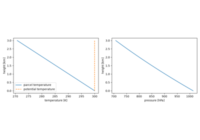
Siméon Denis Poisson showed that a gas compressed or expanded without heat
exchange keeps T p^(-R/c_p) constant. Combined with hydrostatic balance, a
rising dry parcel cools at g / c_p, close to 10 K per kilometre.
Implementation: dry_adiabatic_lapse_rate()
and simulate_dry_ascent(), which integrates
the temperature and pressure of a parcel rising at constant speed. The example
checks the linear cooling and the constant potential temperature.
References: S. D. Poisson, “Sur la chaleur des gaz et des vapeurs,” Annales de Chimie et de Physique 23 (1823): 337-352.
1844 – Magnus’s Vapour-Pressure Formula#
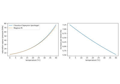
Gustav Magnus measured the pressure of water vapour in equilibrium with liquid water from below freezing to boiling, and fitted it with an exponential in temperature. Clausius derived the same shape from thermodynamics in 1850. The saturation pressure rises by 6-7% per kelvin, so warm air can hold much more water than cold air.
Implementation: saturation_vapor_pressure(),
in the constant-latent-heat Clausius-Clapeyron form, and
relative_humidity(). The example compares it
with a modern Magnus fit.
References: G. Magnus, “Versuche über die Spannkräfte des Wasserdampfs,” Annalen der Physik und Chemie 137 (1844): 225-247.
1857 – Buys Ballot’s Law#
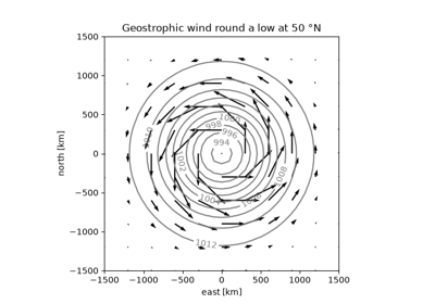
Christophorus Buys Ballot compared simultaneous barometer readings and winds across the Netherlands. In the Northern Hemisphere, with your back to the wind, low pressure is on your left. The wind blows along the isobars, not down the pressure gradient: it is close to geostrophic balance between the pressure gradient and the Coriolis force.
Implementation: geostrophic_speed(). The
example checks that the wind round a low is perpendicular to the gradient and
keeps the low on its left.
References: C. H. D. Buys Ballot, “Note sur le rapport de l’intensité et de la direction du vent avec les écarts simultanés du baromètre,” Comptes Rendus de l’Académie des Sciences 45 (1857): 765-768.
1888 – von Bezold’s Potential Temperature#
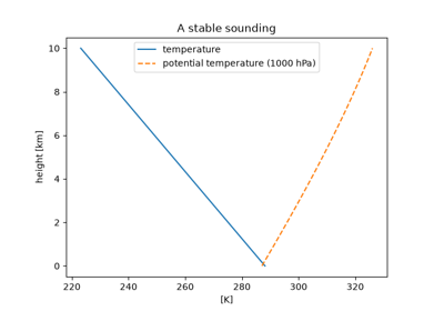
Wilhelm von Bezold named the temperature a sample of air would reach if brought adiabatically to a standard pressure. It does not change when dry air rises or sinks, so it labels air masses and measures static stability: the column is stable where it increases with height.
Implementation: potential_temperature()
and temperature_from_potential().
References: W. von Bezold, “Zur Thermodynamik der Atmosphäre,” Sitzungsberichte der Königlich Preussischen Akademie der Wissenschaften zu Berlin (1888): 485-522.
1902 – Teisserenc de Bort’s Stratosphere#
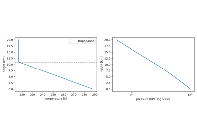
Léon Teisserenc de Bort launched hundreds of unmanned sounding balloons from his observatory at Trappes. Above about 11 km the temperature stopped falling. Richard Assmann reported the same from Berlin that year. The layer above was named the stratosphere and its lower boundary the tropopause.
Implementation: two_layer_temperature()
(new). The example integrates hydrostatic balance through the profile and
recovers the standard-atmosphere pressure at 11 km.
References: L. Teisserenc de Bort, “Variations de la température de l’air libre dans la zone comprise entre 8 km et 13 km d’altitude,” Comptes Rendus de l’Académie des Sciences 134 (1902): 987-989.
1904 – Bjerknes’s Forecasting Programme#
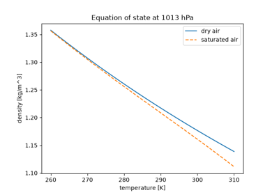
Vilhelm Bjerknes argued that forecasting is an initial-value problem of mechanics and physics. Seven variables (pressure, density, temperature, humidity and three wind components) obey seven equations: three of motion, continuity, the equation of state, and the conservation of heat and of water. The equation of state is the diagnostic link, and with the virtual temperature it applies to moist air.
Implementation: dry_air_density() and
virtual_temperature(). The example checks
that the moist density equals the sum of Dalton’s partial densities.
References: V. Bjerknes, “Das Problem der Wettervorhersage, betrachtet vom Standpunkte der Mechanik und der Physik,” Meteorologische Zeitschrift 21 (1904): 1-7.
1920 – Richardson’s Turbulence Criterion#
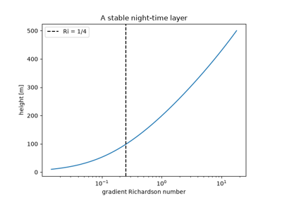
Lewis Fry Richardson asked when wind shear can keep a stably stratified layer
turbulent. Turbulence must lift dense air against buoyancy, at a rate set by
N^2, with energy drawn from the shear. The ratio of the two, now called
the Richardson number, decides the outcome. Miles and Howard proved in 1961
that a stratified shear flow can be unstable only where it falls below 1/4.
Implementation: richardson_number()
(new).
References: L. F. Richardson, “The supply of energy from and to atmospheric eddies,” Proceedings of the Royal Society of London A 97 (1920): 354-373.
1922 – Richardson’s Numerical Forecast#
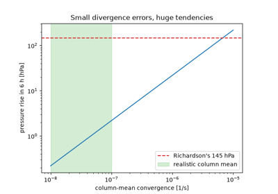
Richardson then carried out Bjerknes’s programme by hand. From observations of 20 May 1910 he computed a six-hour forecast for two grid points over Germany and predicted a surface pressure rise of 145 hPa. The error came mostly from the divergence: the pressure tendency is the column-mean divergence times the surface pressure, and small errors in the winds give a column mean far larger than the true one.
Implementation: surface_pressure_tendency()
(new).
References: L. F. Richardson, Weather Prediction by Numerical Process (Cambridge: Cambridge University Press, 1922).
1925 – Väisälä and Brunt’s Buoyancy Frequency#
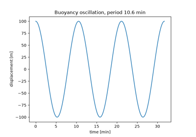
Vilho Väisälä, and independently David Brunt in 1927, showed that a parcel
displaced vertically in stable air oscillates about its level with angular
frequency N = sqrt(g / theta * dtheta/dz). In the troposphere the period
is about ten minutes. Where N^2 is negative the parcel accelerates away
instead.
Implementation: brunt_vaisala_squared().
The example integrates the parcel equation and recovers the period.
References: V. Väisälä, “Über die Wirkung der Windschwankungen auf die Pilotbeobachtungen,” Commentationes Physico-Mathematicae 2, no. 19 (1925); D. Brunt, “The period of simple vertical oscillations in the atmosphere,” Quarterly Journal of the Royal Meteorological Society 53 (1927): 30-32.
1939 – Rossby’s Planetary Waves#
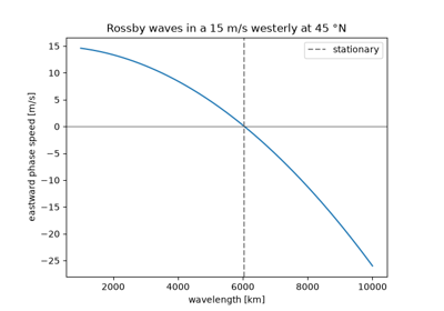
Carl-Gustaf Rossby explained the slow drift of the large troughs and ridges
in the westerlies. Because the Coriolis parameter grows northward at the rate
beta, a vorticity wave moves westward relative to the wind at
beta / k^2. Long waves are stationary or move westward, and a westerly
U has the stationary wavelength 2 pi sqrt(U / beta).
Implementation: rossby_wave_speed()
(new) and rossby_number(), which
confirms that these waves are close to geostrophic balance.
References: C.-G. Rossby and collaborators, “Relation between variations in the intensity of the zonal circulation of the atmosphere and the displacements of the semi-permanent centers of action,” Journal of Marine Research 2 (1939): 38-55.
1950 – Charney, Fjørtoft and von Neumann’s ENIAC Forecast#
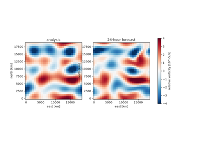
Jule Charney, Ragnar Fjørtoft and John von Neumann ran the first computer weather forecasts on the ENIAC. They forecast only the vorticity of a nondivergent barotropic flow. That equation filters out the gravity waves and divergence errors that ruined Richardson’s forecast, and its 24-hour forecasts of the 500 hPa flow had realistic skill.
Implementation: simulate_barotropic_vorticity()
(new), a pseudo-spectral integration on a doubly periodic beta plane. The
example checks that a single mode moves at Rossby’s speed and that a mix of
modes keeps its enstrophy.
References: J. G. Charney, R. Fjørtoft and J. von Neumann, “Numerical integration of the barotropic vorticity equation,” Tellus 2 (1950): 237-254.
Charney, Fjørtoft and von Neumann’s ENIAC forecast (1950)
See also#
Atmosphere: units, equations and validation for conventions, equations and checks.