History#

“It was found that the wave functions […] in a periodic potential have exactly the form of a modulated plane wave.” – F. Bloch, 1928

A chronology of the breakthroughs behind Tight-Binding theory, from Bloch’s 1928 theorem to the strain-engineered and non-Hermitian lattices of the 2010s. Every stop below has a pointer to the corresponding tbkit functionality and a short, runnable, numerically-verified example in examples/ – nothing here is asserted without also being checked in code.

1928 – Bloch’s Theorem and Band Theory #

F. Bloch showed that the eigenstates of a single electron in a perfectly periodic crystal potential \(V(\mathbf{r}) = V(\mathbf{r} + \mathbf{R})\) take the form

\[\psi_{n\mathbf{k}}(\mathbf{r}) = e^{i\mathbf{k}\cdot\mathbf{r}}\, u_{n\mathbf{k}}(\mathbf{r}), \qquad u_{n\mathbf{k}}(\mathbf{r} + \mathbf{R}) = u_{n\mathbf{k}}(\mathbf{r}),\]

turning the Schrodinger equation for an infinite solid into a finite eigenvalue problem \(H(\mathbf{k})u_{n\mathbf{k}} = E_n(\mathbf{k}) u_{n\mathbf{k}}\) at each crystal momentum \(\mathbf{k}\), periodic on the Brillouin zone torus. This single idea – that a crystal’s electronic structure decomposes into bands \(E_n(\mathbf{k})\) – is the foundation every model in tbkit is built on.

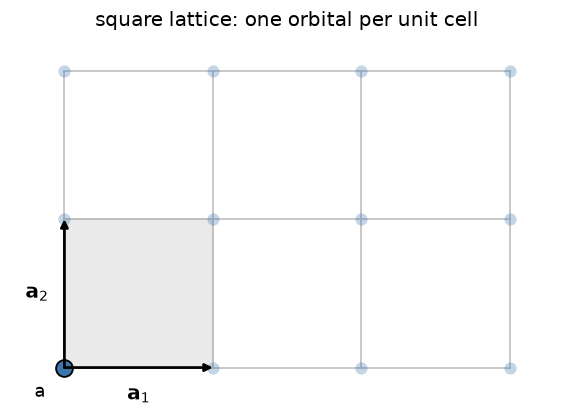
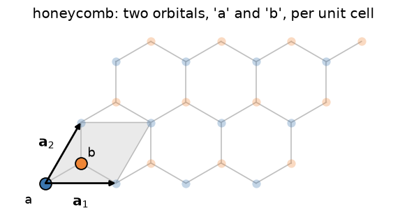
Everything below starts from the same two ingredients: a unit cell (the motif, drawn solid and labelled) and the primitive vectors \(\mathbf{a}_i\) that repeat it. The shaded parallelogram is one unit cell; every faded site is a copy of a solid one, translated by some \(\mathbf{R} = n_1\mathbf{a}_1 + n_2\mathbf{a}_2\).

Implementation: tbkit.kspace.KSpace builds \(H(\mathbf{k})\) directly by Bloch-summing real-space hoppings tagged by which neighboring unit cell they connect to; get_bands(), k_path(), and mesh_bands() diagonalize it at a point, along a path, or over the whole Brillouin zone. tbkit.kspace.reciprocal_vectors() gives the dual lattice vectors \(\mathbf{b}_i\) (\(\mathbf{a}_i\cdot\mathbf{b}_j = 2\pi\delta_{ij}\)) that the Brillouin zone is built from.

References: F. Bloch, “Uber die Quantenmechanik der Elektronen in Kristallgittern,” Z. Phys. 52, 555-600 (1929).

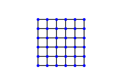
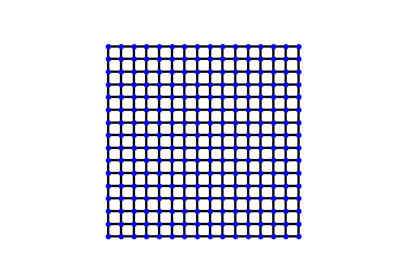
The Square Lattice: Bloch’s Theorem in its Simplest Form

The Square Lattice: Bloch's Theorem in its Simplest Form

1928/1960 – Bloch Oscillations and the Wannier-Stark Ladder #

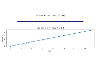
Bloch pointed out an immediate, counterintuitive consequence of his own theorem: a uniform force on an electron in a periodic lattice does not uniformly accelerate it, the way it would in free space. Instead, Bloch’s argument and its later formalization by G. Wannier show the electron oscillates periodically in real space, with period \(T_B = 2\pi/F\) (\(\hbar=1\)), while the spectrum of the tilted lattice collapses into an exactly evenly spaced ladder,

\[E_n = E_0 + nF, \qquad n \in \mathbb{Z},\]

the Wannier-Stark ladder, with every eigenstate exponentially localized around its own lattice site by the tilt alone – a deterministic cousin of Anderson localization (1958, below). In real crystals scattering happens on a timescale far shorter than \(T_B\), which is why the effect went unobserved for over 60 years; it took artificial semiconductor superlattices, with a far larger effective lattice constant and hence much shorter \(T_B\), to see it directly.

Implementation: a uniform force is exactly a linear onsite potential gradient, so no dedicated function is needed: tbkit.system.System.set_onsite_def() applies it directly, and tbkit.propagation.Propagation (see 1954 below for the general Tight-Binding framework it operates on) evolves a wavepacket under the resulting tilted Hamiltonian.

References: F. Bloch, Z. Phys. 52, 555-600 (1929); G. H. Wannier, “Wave functions and effective Hamiltonian for Bloch electrons in an electric field,” Phys. Rev. 117, 432-439 (1960); experimentally confirmed by C. Waschke et al., “Coherent submillimeter-wave emission from Bloch oscillations in a semiconductor superlattice,” Phys. Rev. Lett. 70, 3319-3322 (1993).

Bloch Oscillations and the Wannier-Stark Ladder

1933 – The Peierls Substitution #

R. Peierls showed how to add a magnetic field to a tight-binding model without abandoning the lattice: each hopping amplitude picks up a phase equal to the line integral of the vector potential along the bond,

\[t_{ij} \to t_{ij}\, e^{i\phi_{ij}}\, ,\qquad \phi_{ij} = \frac{2\pi}{\Phi_0}\int_{\mathbf{r}_i}^{\mathbf{r}_j} \mathbf{A}\cdot d\mathbf{l}\, ,\]

with \(\Phi_0 = h/e\) the flux quantum. Because the phase around any closed loop of bonds is gauge-invariant and equals \(2\pi\) times the flux threading it, this recipe reproduces the Aharonov-Bohm and quantum Hall physics below directly on a lattice, without ever solving the continuum Schrodinger equation in a field.

Implementation: tbkit.system.System.set_peierls_phase() applies an arbitrary phase function (any gauge, any spatial field profile); set_magnetic_field() is a symmetric-gauge convenience wrapper for a uniform field, \(\phi_{ij} = \pi\alpha(x_iy_j - x_jy_i)\) with \(\alpha = B/\Phi_0\).

References: R. Peierls, “Zur Theorie des Diamagnetismus von Leitungselektronen,” Z. Phys. 80, 763-791 (1933).

Aharonov-Bohm Ring: A Magnetic Field on a Lattice

Hofstadter’s Butterfly

Hofstadter's Butterfly

1947 – Wallace’s Tight-Binding Prediction of Graphene #

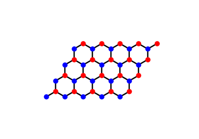
Thirty-nine years before it had a name and fifty-seven years before it was isolated, graphene’s electronic structure was already known: P. R. Wallace worked out the tight-binding band structure of a single honeycomb sheet of carbon (as a stepping stone to understanding bulk graphite) and found something no one had seen in a solid before. The two bands touch at the corners of the hexagonal Brillouin zone, and expanding the dispersion around one such point \(\mathbf{K}\) gives, to leading order,

\[E(\mathbf{K}+\mathbf{q}) \approx \pm \frac{3}{2}\,t\,a\,|\mathbf{q}|\, ,\]

a dispersion that is linear in momentum rather than the usual quadratic \(\hbar^2q^2/2m^*\). Electrons near \(\mathbf{K}\) therefore behave as massless, relativistic (Dirac) particles with an effective speed of light \(v_F = 3ta/2\), decades before “Dirac fermions in condensed matter” became a field in its own right.

The two bands are the two orbitals of the honeycomb unit cell – one on each of the interpenetrating triangular sublattices 'a' and 'b':

Implementation: no new code – this is the same honeycomb tbkit.kspace.KSpace Hamiltonian used throughout this chronology, evaluated at momenta offset from \(\mathbf{K}\) by a small \(\mathbf{q}\).

References: P. R. Wallace, “The Band Theory of Graphite,” Phys. Rev. 71, 622-634 (1947).

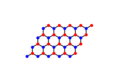
Graphene: Real-Space Flake and Reciprocal-Space Bands

1954 – The Slater-Koster Tight-Binding Framework #

J. Slater and G. Koster showed how to build realistic band structures from a minimal empirical basis: a linear combination of atomic orbitals (LCAO), with hopping matrix elements between neighboring orbitals as fitting parameters rather than computed from first principles. This traded first-principles rigor for tractability and physical transparency, and remains the standard language for model-building in condensed matter theory – it is, in effect, the specification tbkit itself implements: define a unit cell of orbitals, define hoppings between them, and let the code Bloch-sum or diagonalize the result.

Implementation: tbkit.lattice.Lattice (the unit cell and its translations), tbkit.system.System (finite, real-space Hamiltonians) and tbkit.kspace.KSpace (periodic, reciprocal-space Hamiltonians) are exactly this LCAO philosophy, general enough to cover every other model in this chronology. tbkit.lattices collects several standard unit cells (chain, square, triangular, honeycomb, kagome, Lieb) ready to use instead of specifying unit_cell/prim_vec by hand.

References: J. C. Slater and G. F. Koster, “Simplified LCAO Method for the Periodic Potential Problem,” Phys. Rev. 94, 1498-1524 (1954).

Flat-Band Lattices: Kagome and Lieb

1958 – Anderson Localization #

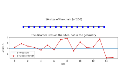
P. Anderson showed that quenched, random disorder is not a small perturbative correction to a metal’s conductivity but can halt transport outright: interference between all the scattering paths off a random potential exponentially localizes the electronic eigenstates, turning a metal into an insulator with no gap and no broken symmetry. Anderson’s own argument established this for strong enough disorder; the scaling theory of Abrahams, Anderson, Licciardello, and Ramakrishnan sharpened it two decades later to the statement that in one and two dimensions every state localizes at any nonzero disorder strength, so that only in three dimensions is there a genuine metal-insulator transition at finite disorder. A localized state’s character is diagnosed by its Inverse Participation Ratio,

\[\mathrm{IPR}_n = \frac{\sum_i|\psi_i^{(n)}|^4}{\left(\sum_i|\psi_i^{(n)}|^2\right)^2}\, ,\]

which is \(O(1/N)\) for a state spread over all \(N\) sites (extended) and \(O(1)\) for a state pinned to a handful of them (localized).

Implementation: tbkit.system.System.set_onsite_dis() and set_hopping_dis() add uniform random disorder to the onsite energies/hoppings; get_ipr() computes \(\mathrm{IPR}_n\) for every eigenstate.

References: P. W. Anderson, “Absence of Diffusion in Certain Random Lattices,” Phys. Rev. 109, 1492-1505 (1958); E. Abrahams, P. W. Anderson, D. C. Licciardello, and T. V. Ramakrishnan, “Scaling Theory of Localization,” Phys. Rev. Lett. 42, 673-676 (1979).

Anderson Localization

1959 – The Aharonov-Bohm Effect #

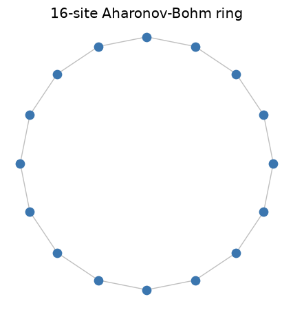
Y. Aharonov and D. Bohm pointed out a startling consequence of quantum mechanics: a charged particle’s phase is affected by the vector potential \(\mathbf{A}\) even in a region where the magnetic field \(\mathbf{B}=\nabla\times\mathbf{A}\) itself vanishes identically – only the enclosed flux \(\Phi = \oint\mathbf{A}\cdot d\mathbf{l}\) matters, and only modulo the flux quantum \(\Phi_0\). On a ring threaded by flux \(\Phi\), this makes the energy spectrum exactly periodic in \(\Phi\) with period \(\Phi_0\).

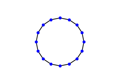
A ring is not a Bravais lattice, so its sites are placed by hand – the flux that matters is the one enclosed by the polygon they span:

Implementation: directly reproduced by tbkit.system.System.set_magnetic_field() (see 1933 above) applied to a ring-shaped Lattice.

References: Y. Aharonov and D. Bohm, “Significance of Electromagnetic Potentials in the Quantum Theory,” Phys. Rev. 115, 485-491 (1959).

Aharonov-Bohm Ring: A Magnetic Field on a Lattice

1930/2005 – Landau Levels: From Free Electrons to Graphene’s Dirac Fermions #

L. Landau showed in 1930 that a charged particle confined to a plane under a uniform perpendicular magnetic field has a spectrum that collapses from a continuum into a ladder of discrete, macroscopically degenerate levels – Landau levels – each level’s degeneracy set purely by the number of flux quanta threading the sample. Applied to a lattice via the Peierls substitution above, at weak field (magnetic length much larger than the lattice spacing) the same quantization survives near a band’s parabolic edge, evenly spaced by the cyclotron frequency \(\omega_c = eB/m^*\),

\[E_n = E_0 + \hbar\omega_c\left(n+\tfrac12\right), \qquad n = 0, 1, 2, \dots\]

Seventy-five years later, K. Novoselov, A. Geim, and coworkers, and independently Y. Zhang, Y.-W. Tan, H. Stormer, and P. Kim, measured graphene’s Landau levels directly and found something Landau’s original theory never anticipated: because graphene’s low-energy electrons obey Wallace’s linear (massless-Dirac) dispersion above rather than the usual parabolic one, the ladder is spaced by \(\sqrt{n}\) rather than \(n\), and centered on an exact zero-energy level present at any field strength – a direct experimental fingerprint, via the resulting anomalous quantum Hall sequence, that graphene’s charge carriers behave as massless Dirac fermions rather than ordinary electrons.

\[E_n = \mathrm{sign}(n)\, v_F\sqrt{2\hbar e B|n|}, \qquad n = 0, \pm1, \pm2, \dots\]

The two ladders below are the same field applied to two different finite flakes – a square lattice (parabolic band edge) and a graphene flake (linear Dirac cone):

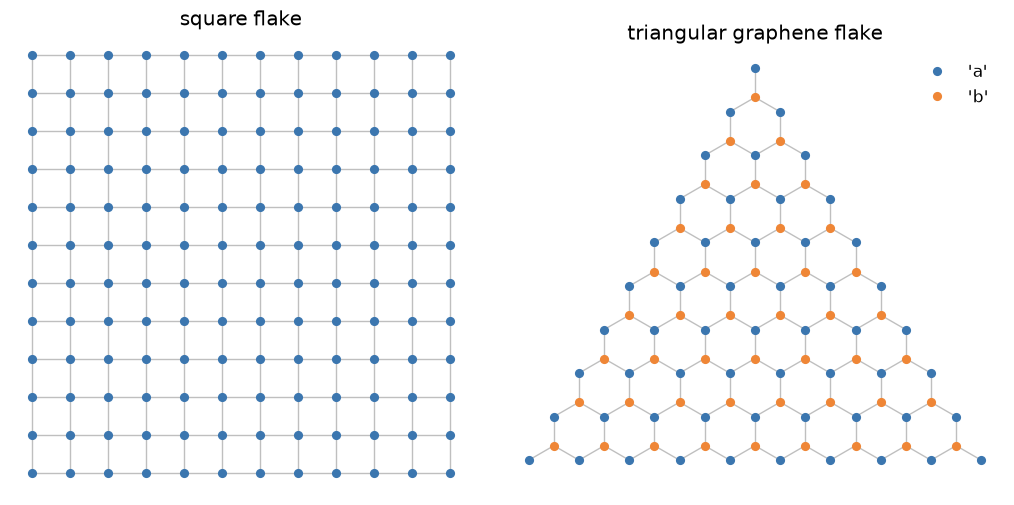
Implementation: both ladders come from exactly the same tbkit.system.System.set_magnetic_field() used throughout this chronology, applied to two different finite flakes: a square lattice (parabolic band edge) and a graphene flake built from tbkit.graphene.GrapheneLattice (linear Dirac dispersion). No dedicated Landau-level function is needed – the quantization is an emergent, weak-field limit of the same Peierls-substituted Hamiltonian Hofstadter’s full flux sweep uses below.

References: L. Landau, “Diamagnetismus der Metalle,” Zeitschrift fur Physik 64, 629-637 (1930); K. S. Novoselov, A. K. Geim, S. V. Morozov, D. Jiang, M. I. Katsnelson, I. V. Grigorieva, S. V. Dubonos, and A. A. Firsov, “Two-Dimensional Gas of Massless Dirac Fermions in Graphene,” Nature 438, 197-200 (2005); Y. Zhang, Y.-W. Tan, H. L. Stormer, and P. Kim, “Experimental Observation of the Quantum Hall Effect and Berry’s Phase in Graphene,” Nature 438, 201-204 (2005).

Example: examples/magnetic_field/plot_landau_levels.py builds a 60x60 square-lattice flake and a 1936-site triangular graphene flake at the same weak flux, confirms exact particle-hole symmetry in both (the Peierls substitution preserves bipartite chiral symmetry), confirms the square lattice’s lowest 72 nearly-degenerate states average to within 15% of the predicted \(E_0+\omega_c/2\), and confirms graphene’s clean n=1 plateau (102 states) matches the predicted \(v_F\sqrt{2eB}\) to within 1%.

Landau Levels: Square Lattice vs. Graphene

1976 – Hofstadter’s Butterfly #

D. Hofstadter solved the tight-binding square lattice threaded by a continuously varying flux per plaquette \(\alpha = p/q\) (in units of \(\Phi_0\)) and found a spectrum of startling, self-similar complexity: at each rational flux \(p/q\), the band splits into \(q\) sub-bands, and plotting energy against \(\alpha\) traces out a fractal, recursively structured pattern now known as Hofstadter’s butterfly – one of the earliest and most famous numerically-discovered fractals in physics, and a direct illustration of how sensitively a Bloch spectrum can depend on a magnetic field via the Peierls substitution above.

Implementation: the same tbkit.system.System.set_magnetic_field() used for the Aharonov-Bohm ring, swept continuously over a finite 2D flake.

References: D. R. Hofstadter, “Energy levels and wave functions of Bloch electrons in rational and irrational magnetic fields,” Phys. Rev. B 14, 2239-2249 (1976).

Hofstadter’s Butterfly

Hofstadter's Butterfly

1979 – The Su-Schrieffer-Heeger (SSH) Model #

Su, Schrieffer, and Heeger showed that a 1D dimerized chain – alternating intracell (\(v\)) and intercell (\(w\)) bonds, modeling polyacetylene – hosts domain-wall solitons. Cut open into a finite chain, the same physics produces a pair of protected, exponentially localized zero-energy states, one at each end, whenever \(w>v\). It is the earliest and simplest example of the bulk-boundary correspondence that would come to define topological band theory: a bulk property predicting the existence of boundary modes.

\[\begin{split}H(k) = \begin{pmatrix} 0 & v + w\,e^{-ik} \\ v + w\,e^{ik} & 0 \end{pmatrix}, \qquad E_\pm(k) = \pm|v + w\,e^{-ik}|\, .\end{split}\]

Which phase the chain is in is visible in the geometry: it is set by whether the chain is cut so that the weak bond or the strong one sits at the end.

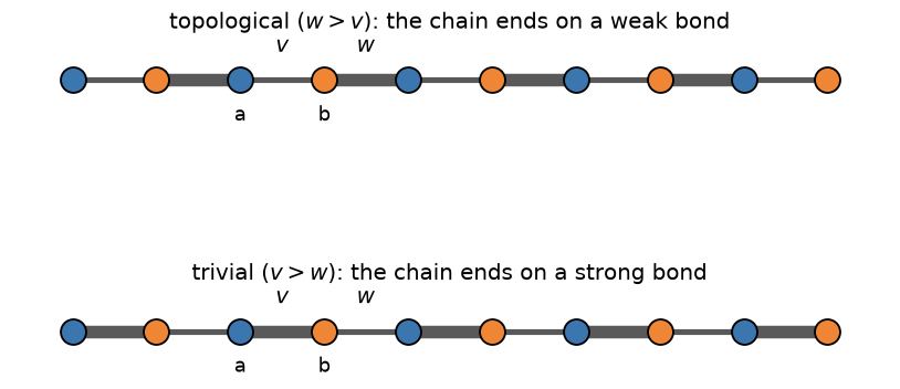
The bulk gap \(2\min_k|v+we^{-ik}| = 2|v-w|\) closes only at \(v=w\); for \(v<w\) the chain is topological (protected zero-energy edge modes under open boundaries), and for \(v>w\) it is trivial (no edge modes).

Implementation: built directly from tbkit.kspace.KSpace (the Bloch form above) and tbkit.system.System.set_hopping_manual() (the open, real-space chain exposing the edge modes) – no dedicated SSH function is needed, since the general hopping-list framework already covers it exactly.

References: W. P. Su, J. R. Schrieffer, and A. J. Heeger, “Solitons in Polyacetylene,” Phys. Rev. Lett. 42, 1698-1701 (1979).

The SSH Model: Bulk-Boundary Correspondence

1982 – The TKNN Invariant #

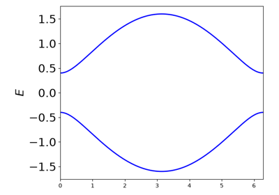
Thouless, Kohmoto, Nightingale, and den Nijs (TKNN) showed that a 2D band’s quantized Hall conductance is a topological invariant: the integral of its Berry curvature \(\Omega(\mathbf{k})\) over the Brillouin zone,

\[C = \frac{1}{2\pi}\int_{\mathrm{BZ}} \Omega(\mathbf{k})\, d^2k \in \mathbb{Z}\, ,\]

now called the (first) Chern number. Because \(C\) can only change when a bulk energy gap closes, it is invariant under any smooth, gap-preserving perturbation – the single idea that turned “band theory” into “topological band theory,” and the direct theoretical explanation for why the integer quantum Hall effect (measured by von Klitzing two years earlier) is quantized with such extraordinary precision.

Implementation: tbkit.kspace.KSpace.berry_curvature() computes \(\Omega(\mathbf{k})\) over a Brillouin-zone mesh by the gauge-invariant Fukui-Hatsugai-Suzuki lattice method (the phase of a product of overlaps between neighboring-plaquette occupied subspaces, which needs no smooth gauge choice for \(u_{n\mathbf{k}}\) at all); chern_number() is its sum divided by \(2\pi\), returning an integer to within the mesh resolution.

References: D. J. Thouless, M. Kohmoto, M. P. Nightingale, and M. den Nijs, “Quantized Hall Conductance in a Two-Dimensional Periodic Potential,” Phys. Rev. Lett. 49, 405-408 (1982).

The Haldane Model: Berry Curvature and a Topological Phase Transition

1983 – The Thouless Quantum Pump #

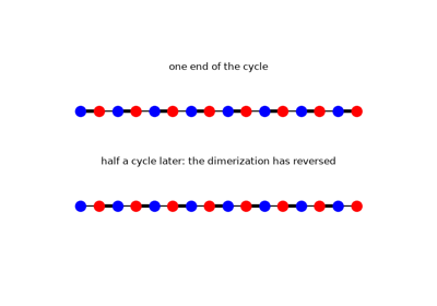
Thouless asked what the TKNN invariant means for a 1D system rather than a 2D one, and found a direct physical answer: if a 1D insulator’s Hamiltonian is cycled slowly and periodically through a parameter \(\phi\) (a pump cycle) back to itself, the charge transported across any cross-section over one full cycle is exactly quantized,

\[Q = \int_0^{2\pi} \frac{dP}{d\phi}\, d\phi \in \mathbb{Z}\, ,\]

an integer number of electrons per cycle, regardless of how the cycle is driven – provided the bulk gap never closes. The reason is exactly the TKNN argument one dimension down: treating the pump parameter \(\phi\) as a second, synthetic crystal momentum turns the 1D pump into a 2D Chern insulator on the \((k,\phi)\) torus, with \(Q\) equal to its Chern number. The idea now underlies “topological pumps” realized with cold atoms in modulated optical lattices, decades after the original proposal.

Implementation: no new code – a pump is simply an ordinary tbkit.kspace.KSpace Bloch Hamiltonian built with the pump parameter as a second reciprocal direction, so chern_number() (1982, above) applies directly and needs no special-casing for the synthetic-dimension trick.

References: D. J. Thouless, “Quantization of particle transport,” Phys. Rev. B 27, 6083-6087 (1983); M. J. Rice and E. J. Mele, “Elementary Excitations of a Linearly Conjugated Diatomic Polymer,” Phys. Rev. Lett. 49, 1455-1459 (1982) (the pumped model itself).

The Thouless Quantum Pump (Rice-Mele Model)

1988 – The Haldane Model #

D. Haldane asked whether the integer quantum Hall effect requires a net magnetic field at all – and showed it does not. His model threads complex second-neighbor hopping \(t_2e^{i\phi}\) through a honeycomb lattice in a pattern with zero net flux per unit cell (opposite chirality on the two sublattices), yet nonzero local curvature that breaks time-reversal symmetry. The result is a Chern insulator, \(C=\pm1\), from lattice-scale “orbital magnetism” alone – the first concrete example of what is now called the quantum anomalous Hall effect, and the direct template for the Kane-Mele model below.

Implementation: built directly from tbkit.kspace.KSpace’s general complex-hopping machinery (no dedicated function needed): real nearest-neighbor hopping plus complex, sublattice-alternating next-nearest-neighbor hopping, evaluated with chern_number().

References: F. D. M. Haldane, “Model for a Quantum Hall Effect without Landau Levels,” Phys. Rev. Lett. 61, 2015-2018 (1988).

The Haldane Model: Berry Curvature and a Topological Phase Transition

1989 – Lieb’s Theorem and Flat-Band Lattices #

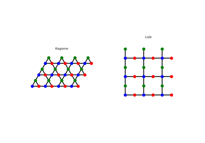
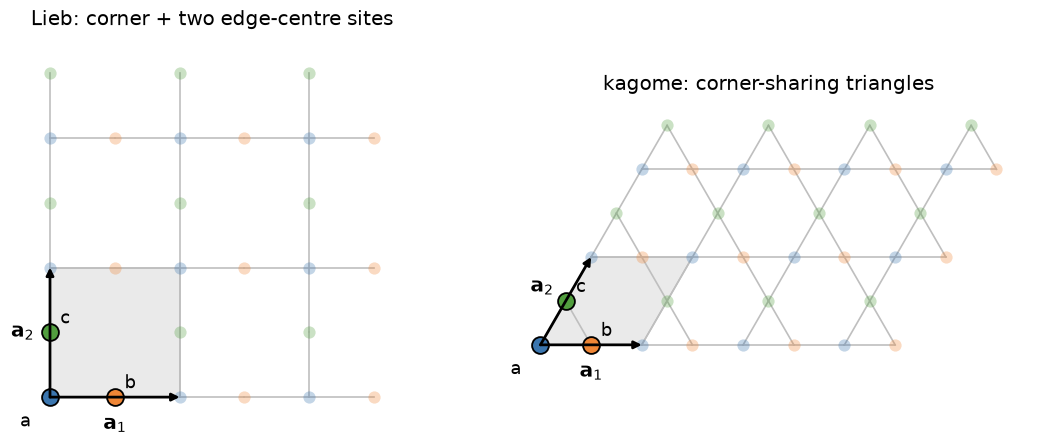
E. Lieb proved one of the few rigorous, non-perturbative results about the many-body Hubbard problem: on a bipartite lattice with unequal numbers of sites on its two sublattices \(A\) and \(B\), the half-filled ground state has total spin exactly \(S = \bigl||A|-|B|\bigr|/2\), for any repulsion \(U>0\) – ferrimagnetic order, with a net moment, derived without approximation. The lattice Lieb used to prove it – a square lattice with an extra site at the midpoint of every bond, so three sites per unit cell split two-to-one between the sublattices – turns out to have an exactly flat (dispersionless) single-particle band already at the noninteracting level, from destructive interference confining an eigenstate to a single 4-site plaquette with zero amplitude everywhere else; the kagome lattice shares the same flat-band mechanism on a different geometry. A flat band’s macroscopic, noninteracting degeneracy is exactly the extreme limit in which arbitrarily weak interactions dominate – the underlying reason flat-band lattices remain an active route to engineered strong correlation and (on kagome, with further ingredients) topological flat-band physics.

Both lattices owe their flat band to the same thing – a unit cell with more sites than the number of independent ways an electron can leave it:

Implementation: tbkit.lattices.lieb() and tbkit.lattices.kagome() provide both lattices’ unit cells directly, ready for KSpace.

References: E. H. Lieb, “Two Theorems on the Hubbard Model,” Phys. Rev. Lett. 62, 1201-1204 (1989).

Flat-Band Lattices: Kagome and Lieb

2000/2011 – A Topological Flat Band on the Kagome Lattice #

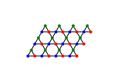
K. Ohgushi, S. Murakami, and N. Nagaosa showed in 2000 that a canted (non-coplanar) magnetic texture on the kagome lattice, via the scalar spin chirality its itinerant electrons pick up hopping around each elementary triangle, acts on those electrons exactly like a complex nearest-neighbor hopping amplitude \(te^{i\phi}\) – breaking time-reversal symmetry with no net magnetic field, the kagome counterpart of Haldane’s honeycomb construction above. That complex phase gaps the flat band’s symmetry-protected touching point with the lattice’s middle band (above), leaving the (no longer exactly flat) lower band a genuine Chern insulator. Eleven years later, three independent 2011 papers (Tang, Mei, and Wen; Sun, Gu, Katsura, and Das Sarma; Neupert, Santos, Chamon, and Mudry) generalized the same idea into a broader research program: engineer lattice models whose lowest band is simultaneously nearly flat and topologically nontrivial, as a route to fractional-quantum-Hall-like physics – a fractional Chern insulator – entirely without Landau levels or a net magnetic field.

Implementation: tbkit.lattices.kagome() with every nearest-neighbor hopping set to the same complex amplitude \(te^{i\phi}\) (rather than the real, uniform \(t\) used above) via tbkit.kspace.KSpace.set_hopping(); chern_number() and berry_curvature() (1982 above) diagnose the resulting band’s topology exactly as for the Haldane model.

References: K. Ohgushi, S. Murakami, and N. Nagaosa, “Spin Anisotropy and Quantum Hall Effect in the Kagome Lattice: Chiral Spin State Based on a Ferromagnet,” Phys. Rev. B 62, R6065-R6068 (2000); E. Tang, J.-W. Mei, and X.-G. Wen, “High-Temperature Fractional Quantum Hall States,” Phys. Rev. Lett. 106, 236802 (2011); K. Sun, Z. Gu, H. Katsura, and S. Das Sarma, “Nearly Flatbands with Nontrivial Topology,” Phys. Rev. Lett. 106, 236803 (2011); T. Neupert, L. Santos, C. Chamon, and C. Mudry, “Fractional Quantum Hall States at Zero Magnetic Field,” Phys. Rev. Lett. 106, 236804 (2011).

Example: examples/topology/plot_kagome_chern_band.py confirms the flat band and middle band are exactly degenerate at \(\Gamma\) when \(\phi=0\), confirms a real gap (larger than 0.3t) opens across the whole Brillouin zone once \(\phi\ne0\), and confirms the resulting three bands’ Chern numbers are exactly \(-1, 0, +1\) – summing to zero, as they must.

A Topological Flat Band on the Kagome Lattice

2004 – Isolation of Graphene #

A. Geim, K. Novoselov, and coworkers mechanically exfoliated a single atomic layer of carbon from graphite, producing the first genuinely 2D crystal. Graphene’s low-energy quasiparticles obey a massless relativistic (Dirac) equation rather than the usual Schrodinger equation: expanding the honeycomb-lattice \(H(\mathbf{k})\) near either inequivalent Brillouin-zone corner \(K\), \(K'\) gives a linear dispersion, \(E(\mathbf{k}) = \pm\hbar v_F|\mathbf{k}|\), with the two bands touching at exactly zero energy – turning a tabletop condensed matter experiment into a laboratory for relativistic quantum phenomena, and putting the honeycomb lattice, and Haldane’s sixteen-year old model built on it, at the center of the field. Geim and Novoselov shared the 2010 Nobel Prize in Physics for this work.

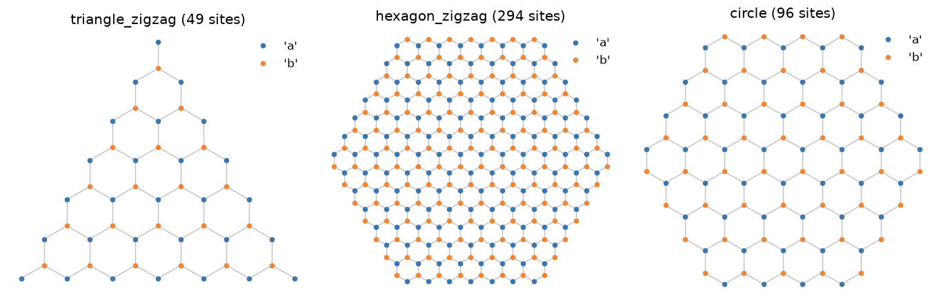
Implementation: tbkit.lattices.honeycomb(), or the equivalent hand-built unit cell used throughout this package’s graphene examples; tbkit.graphene.GrapheneLattice additionally provides ready-made finite flakes of several shapes and terminations (triangular/hexagonal, zigzag/armchair).

References: K. S. Novoselov, A. K. Geim, S. V. Morozov, D. Jiang, Y. Zhang, S. V. Dubonos, I. V. Grigorieva, and A. A. Firsov, “Electric Field Effect in Atomically Thin Carbon Films,” Science 306, 666-669 (2004).

Graphene: Real-Space Flake and Reciprocal-Space Bands

2005-2007 – The Kane-Mele Model and the Quantum Spin Hall Effect #

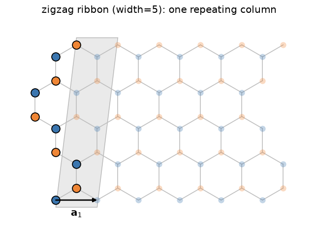
C. Kane and E. Mele showed in 2005 that adding intrinsic spin-orbit coupling to graphene – two time-reversed copies of Haldane’s model, one per spin, with opposite Chern number so the total Chern number vanishes – produces a new, time-reversal-symmetric topological phase protected by a \(\mathbb{Z}_2\) (rather than integer) invariant: the quantum spin Hall effect. A finite ribbon of this model hosts a Kramers pair of helical, counter-propagating, spin-momentum-locked edge states that cannot be gapped out by any time-reversal-symmetric perturbation – immune to backscattering because a spin-up right-mover has no same-momentum, same-spin partner to scatter into. Konig et al. observed exactly this two-terminal quantized conductance in HgTe/CdTe quantum wells in 2007, the first experimentally realized topological insulator of any kind.

Edge states need an edge, so the model is cut into a ribbon: periodic along one primitive vector, finite along the other. The shaded column is the repeating unit; the ribbon is that column tiled sideways, and its two open edges are where the helical states live.

Implementation: tbkit.kspace.KSpace constructed with spin=True gives every site a spin-1/2 degree of freedom, with set_hopping()/set_onsite() accepting 2x2 (Pauli) matrices – built from tbkit.kspace.PAULI – for spin-dependent terms such as Kane-Mele’s \(i\lambda_{SO}\sigma_z\) next-nearest-neighbor coupling or Rashba spin-orbit coupling; tbkit.kspace.ribbon() cuts the open, finite-width ribbon that exposes the helical edge states directly in the spectrum.

References: C. L. Kane and E. J. Mele, “Z2 Topological Order and the Quantum Spin Hall Effect,” Phys. Rev. Lett. 95, 146802 (2005); C. L. Kane and E. J. Mele, “Quantum Spin Hall Effect in Graphene,” Phys. Rev. Lett. 95, 226801 (2005); M. Konig et al., “Quantum Spin Hall Insulator State in HgTe Quantum Wells,” Science 318, 766-770 (2007).

Edge States on Ribbons

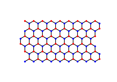
2010 – Strain as a Gauge Field: Pseudo-Magnetic Fields #

F. Guinea, M. Katsnelson, and A. Geim pointed out that graphene offers a way to build a magnetic field out of nothing but mechanical deformation. Straining the sheet changes its bond lengths and therefore its hopping amplitudes, and near the Dirac point a smooth modulation of the three nearest-neighbor hoppings enters the Dirac equation in precisely the slot a vector potential occupies: it displaces the Dirac cone in momentum space rather than shifting its energy. A triaxial strain whose modulation grows linearly with distance from the center therefore acts on the electrons as a uniform pseudo-magnetic field,

\[\mathbf{A} = \tfrac{1}{2}B_s(-y,\, x)\, ,\qquad B_s = \beta/2\, ,\]

(\(\beta\) the strain strength in the convention below, \(\hbar=e=a=1\)), quantizing the spectrum into exactly the relativistic ladder \(E_n = \mathrm{sign}(n)v_F\sqrt{2B_s|n|}\) that a real field produces.

What makes this more than an analogy is what is missing. Every hopping stays real, so the Hamiltonian is real, time-reversal symmetry is never broken – and a time-reversal-symmetric Hamiltonian cannot host a genuine magnetic field. The resolution is that the pseudo-field must point the opposite way at the second valley \(\mathbf{K}'\): carriers in the two valleys bend in opposite directions, so the sample carries no net Hall current even while each valley is fully Landau-quantized. Nor is the effect bounded by what a laboratory magnet can deliver, since nothing is being magnetized: Levy and coworkers measured pseudo-Landau levels in strained graphene nanobubbles corresponding to fields above 300 T, an order of magnitude beyond the strongest static fields available anywhere.

Implementation: tbkit.graphene.GrapheneSystem.set_hop_linear_strain() sets every nearest-neighbor bond to \(t_{ij} = t(1 + \tfrac14\beta\, \hat{\boldsymbol\delta}_{ij}\cdot\mathbf{r}_{ij})\), with \(\hat{\boldsymbol\delta}_{ij}\) the bond direction and \(\mathbf{r}_{ij}\) its midpoint – linear triaxial strain, measured from the coordinate origin, so the flake must be centered on it. get_beta_lims() returns the largest strain that still leaves every hopping positive, and get_butterfly() sweeps \(\beta\) across that whole range – the strain analogue of Hofstadter’s flux sweep (1976, above).

References: F. Guinea, M. I. Katsnelson, and A. K. Geim, “Energy gaps and a zero-field quantum Hall effect in graphene by strain engineering,” Nature Physics 6, 30-33 (2010); N. Levy, S. A. Burke, K. L. Meaker, M. Panlasigui, A. Zettl, F. Guinea, A. H. Castro Neto, and M. F. Crommie, “Strain-Induced Pseudo-Magnetic Fields Greater Than 300 Tesla in Graphene Nanobubbles,” Science 329, 544-547 (2010); the strain gauge field itself goes back to H. Suzuura and T. Ando, “Phonons and electron-phonon scattering in carbon nanotubes,” Phys. Rev. B 65, 235412 (2002).

Example: examples/strain/plot_pseudo_magnetic_field.py strains a 1728-site circular graphene flake at \(\beta=-0.05\), confirms the Hamiltonian is exactly real (unlike the complex, Peierls-substituted one it is compared against), and confirms that its bulk states nevertheless bunch onto the first four pseudo-Landau levels \(E_n = \tfrac32 t\sqrt{\beta n}\) to within 3%, with the \(\sqrt{n}\) spacing of a Dirac cone rather than the even spacing of a parabolic band. It then confirms that \(E_1\) tracks \(\sqrt{\beta}\) across a range of strains, and that a real field of the same strength, \(\alpha = B_s/2\pi\), reproduces the same \(E_1\) to within 3% through a complex Hamiltonian.

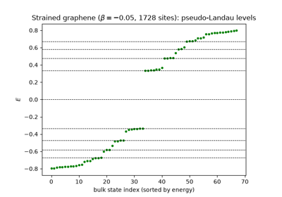
Strain as a Gauge Field: Pseudo-Landau Levels in Graphene

1998/2015 – PT Symmetry, Exceptional Points, and Gain-Loss Lattices #

C. Bender and S. Boettcher overturned a piece of textbook folklore: Hermiticity is sufficient for a real spectrum, but it is not necessary. A Hamiltonian merely symmetric under the combined parity-time operation \(\mathcal{PT}\) can have an entirely real spectrum too. On a lattice this means balanced gain and loss – imaginary onsite energies \(\pm i\gamma\) placed symmetrically on the two sublattices – leaves every eigenvalue real up to a finite threshold in \(\gamma\).

At that threshold the eigenvalues do not cross; they collide and move off into the complex plane as conjugate pairs. The collision point is an exceptional point, and it is unlike any Hermitian degeneracy: the two eigenvectors coalesce as well, so the Hamiltonian loses a dimension of its eigenbasis and stops being diagonalizable altogether. How close a mode has come to that degeneracy is measured by the Petermann factor \(K_n\), introduced decades earlier in laser physics to explain anomalously broad linewidths,

\[K_n = \frac{\langle\psi_L^{n}|\psi_L^{n}\rangle \langle\psi_R^{n}|\psi_R^{n}\rangle} {|\langle\psi_L^{n}|\psi_R^{n}\rangle|^2}\, ,\]

which equals 1 for an orthogonal (Hermitian) eigenbasis and diverges at an exceptional point. None of this is a formal game: gain and loss are the most accessible knobs an optics experimentalist has, and \(\mathcal{PT}\) symmetry breaking was seen directly in coupled optical waveguides in 2010.

Combined with topology it produces an effect with no Hermitian counterpart at all. Chiral symmetry forces each of the SSH model’s zero modes (1979, above) to live entirely on one sublattice, so sublattice gain and loss is felt by them but not by the bulk states, which are spread evenly over both. The topological modes are therefore the first to leave the real axis, picking up energies \(\pm i\gamma\) at any gain at all, while the entire bulk stays real until \(\gamma\) reaches the bulk gap – a way to amplify a topological mode selectively, demonstrated in a chain of dielectric microwave resonators.

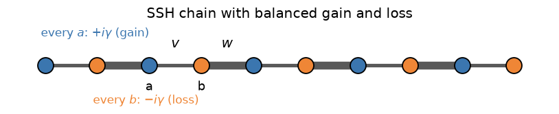
Implementation: tbkit.system.System.set_onsite() accepts complex onsite energies, and get_eig() detects a non-Hermitian Hamiltonian and switches to the general (non-symmetric) eigensolver, with left=True returning the left eigenvectors too; get_petermann() builds \(K_n\) from both sets, and tbkit.plot.Plot.spectrum_complex() plots the real and imaginary parts of the spectrum together.

References: C. M. Bender and S. Boettcher, “Real Spectra in Non-Hermitian Hamiltonians Having PT Symmetry,” Phys. Rev. Lett. 80, 5243-5246 (1998); K. Petermann, “Calculated spontaneous emission factor for double-heterostructure injection lasers with gain-induced waveguiding,” IEEE J. Quantum Electron. 15, 566-570 (1979); C. E. Ruter, K. G. Makris, R. El-Ganainy, D. N. Christodoulides, M. Segev, and D. Kip, “Observation of parity-time symmetry in optics,” Nature Physics 6, 192-195 (2010); H. Schomerus, “Topologically protected midgap states in complex photonic lattices,” Opt. Lett. 38, 1912-1914 (2013); C. Poli, M. Bellec, U. Kuhl, F. Mortessagne, and H. Schomerus, “Selective enhancement of topologically induced interface states in a dielectric resonator chain,” Nat. Commun. 6, 6710 (2015).

Example: examples/non_hermitian/plot_pt_symmetry.py confirms, for a gain-loss dimer, that the spectrum is real and equal to \(\pm\sqrt{t^2-\gamma^2}\) below the exceptional point at \(\gamma=t\), purely imaginary above it, and that the Petermann factor matches \(1/(1-\gamma^2/t^2)\) to machine precision before diverging at the exceptional point itself. It then applies the same gain-loss pattern to a 40-site topological SSH chain and confirms that exactly two states – the edge modes – acquire imaginary parts, at exactly \(\pm i\gamma\), that the amplified one lies entirely on the gain sublattice and the damped one entirely on the loss sublattice, and that the bulk stays real until \(\gamma\) exceeds \(|v-w|\).

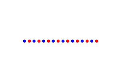
PT Symmetry, Exceptional Points, and a Selectively Amplified Edge Mode