Tutorial#

This walks through tbkit’s pieces in the order you would normally use them: define a lattice, build a real-space Tight-Binding model and diagonalize it, build the same model’s Bloch Hamiltonian in reciprocal space, then layer on more physics (disorder, strain, a magnetic field, spin-orbit coupling, topology, edge states), and on to three dimensions, several orbitals per site, large lattices, transport, interactions, superconductivity, and non-Hermitian and driven systems. Runnable versions of most of this live in the examples/ directory, referenced throughout.

A Tight-Binding Hamiltonian describes electrons hopping between localized orbitals:

\[H = \sum_i \epsilon_i c_i^\dagger c_i + \sum_{i \neq j} t_{ij}\, c_i^\dagger c_j\]

where \(\epsilon_i\) are onsite energies and \(t_{ij}\) are hopping amplitudes between orbitals i and j. Everything in tbkit is about building this matrix (or, in reciprocal space, its Bloch analog \(H(\mathbf{k})\)) and then doing something with it: diagonalizing it, plotting it, evolving a wavepacket under it.

Building a lattice#

tbkit.lattice.Lattice defines the geometry: a unit cell (a list of orbitals, each with a sublattice tag and a position) and one or two primitive vectors:

from tbkit.lattice import Lattice

unit_cell = [{'tag': 'a', 'r0': (0., 0.)}]
prim_vec = [(1., 0.), (0., 1.)]
lat = Lattice(unit_cell=unit_cell, prim_vec=prim_vec)
lat.get_lattice(n1=6, n2=6)   # 6x6 unit cells -> 36 sites

The unit cell is the motif; the primitive vectors say how to repeat it. Here one site per cell repeated on a square grid:

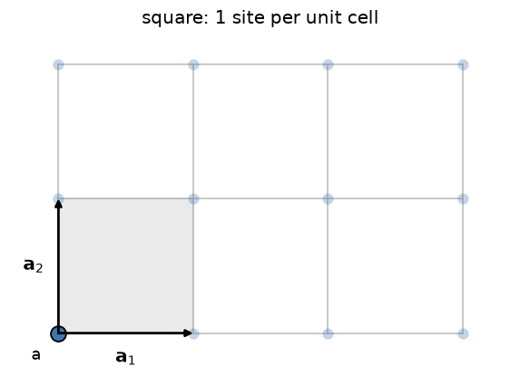
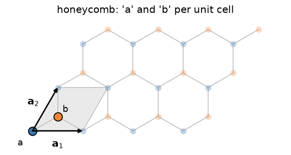
Throughout this page, the shaded parallelogram is the unit cell, the arrows are \(\mathbf{a}_1\) and \(\mathbf{a}_2\), and the sites drawn solid and labelled are the cell’s own orbitals – every faded site is a copy of one of them, translated by some \(\mathbf{R}=n_1\mathbf{a}_1+n_2\mathbf{a}_2\).

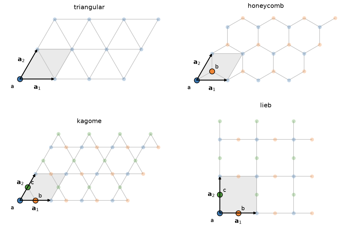
lat.coor now holds every site’s position and tag. Sculpt the shape with methods like remove_sites, ellipse_in/ellipse_out, boundary_line, or by adding/subtracting two lattices (lat1 + lat2). tbkit.lattices has a handful of common lattices (chain, square, triangular, honeycomb, kagome, Lieb) ready to use instead of writing out unit_cell/prim_vec by hand. Their unit cells are what distinguishes them – one site for the square and triangular lattices, two for the honeycomb, three for the kagome and Lieb:

See lat.plot() to look at what you built, and examples/tight_binding/plot_building_finite_lattices.py for many more shapes.

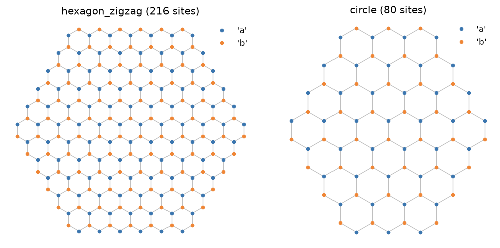
Sculpting works on the finite patch. Cutting a disc out of a honeycomb sheet, for instance:

Real space: build and solve a finite system#

tbkit.system.System takes a Lattice and builds the Hamiltonian from a list of hoppings:

from tbkit.system import System

sys = System(lat)
sys.set_onsite({'a': 0.})
sys.set_hopping([{'n': 1, 't': 1.}])   # nearest-neighbor hopping t=1
sys.get_ham()
sys.get_eig()
print(sys.en)   # eigenenergies, sorted

Hoppings are addressed by neighbor order ('n': 1 is nearest-neighbor, 'n': 2 next-nearest, …; sys.print_distances() lists them), and optionally further filtered by bond angle or by sublattice-pair tag – see tbkit.system.System.set_hopping()’s docstring for the full mini-language. For anything that doesn’t fit that pattern, i,j-indexed hoppings work directly on the actual real-space site indices printed by lat.plot(plt_index=True). Hamiltonians can be Hermitian or, if you fill in both the upper and the lower parts independently (upper_part=True and upper_part=False), non-Hermitian.

tbkit.plot.Plot plots the lattice, the spectrum, sublattice polarization, eigenstate intensities, and the density of states (dos()):

from tbkit.plot import Plot
p = Plot(sys)
p.spectrum()
p.dos(broadening=0.1)

Visualizing a Model: tbkit.plot.Plot

Reciprocal space: Bloch Hamiltonians and band structures#

A finite flake is one way to look at a lattice; the other is to keep it infinite and periodic, and work with its Bloch Hamiltonian \(H(\mathbf{k})\). tbkit.kspace.KSpace builds it from a small set of intra-unit-cell hoppings, each tagged by which neighboring cell (\(\mathbf{R} = n_1\mathbf{a}_1+n_2\mathbf{a}_2\)) it connects to:

from tbkit.kspace import KSpace, reciprocal_vectors
import tbkit.lattices as lattices
import numpy as np

lat = lattices.honeycomb()
gra = KSpace(lat)
gra.set_hopping([{'i': 0, 'j': 1, 'R': (0, 0), 't': 1.},
                        {'i': 0, 'j': 1, 'R': (-1, 0), 't': 1.},
                        {'i': 0, 'j': 1, 'R': (0, -1), 't': 1.}])

Those three dictionaries are exactly the three bonds leaving the cell’s 'a' site: one to the 'b' in the same cell (\(\mathbf{R}=(0,0)\)), and one each to the 'b' of the cells at \(\mathbf{R}=(-1,0)\) and \(\mathbf{R}=(0,-1)\).

Only one representative of each bond is needed – the reverse bond (\(j\to i\), \(\mathbf{R}\to-\mathbf{R}\)) is added automatically as its Hermitian conjugate. Diagonalize at a single k-point with get_ham/LA.eigh, over an explicit set of k-points with get_bands, or along a path through high-symmetry points with k_path (reciprocal_vectors() gives the reciprocal lattice vectors to build that path from):

b1, b2 = (np.array(v) for v in reciprocal_vectors(lat.prim_vec))
Gamma, K, M = np.zeros(2), (b1 - b2)/3, b1/2
gra.k_path([Gamma, K, M, Gamma], nk=60)
fig = gra.plot_bands(node_labels=[r'$\Gamma$', 'K', 'M', r'$\Gamma$'])

high_symmetry_path() recognizes the Bravais lattice and returns a standard path with its labels (here \(\Gamma\)-M-K-\(\Gamma\)):

points, labels = high_symmetry_path(lat)
gra.k_path(points, nk=60)
fig = gra.plot_bands(node_labels=labels)

gra.mesh_bands(nk) samples a uniform mesh over the whole Brillouin zone instead (used internally by plot_dos, and for the topology tools below). See examples/tight_binding/plot_graphene_bands.py. On top of the bands: plot_bands(weights=gra.band_weights('a')) colors them by their weight on a sublattice (fat bands), plot_fermi_surface(E) draws the constant-energy contours, and plot_dos(kernel='tetrahedron') gives the density of states without broadening.

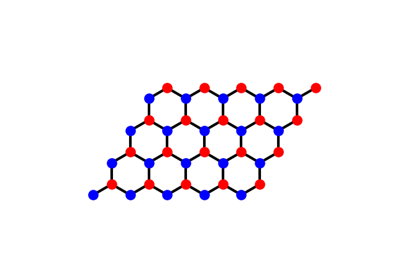
Graphene: Real-Space Flake and Reciprocal-Space Bands

Disorder, strain, and a magnetic field#

On a System, set_onsite_dis/set_hopping_dis add uniform random disorder; GrapheneSystem.set_hop_linear_strain (in tbkit.graphene) applies triaxial strain. An orbital magnetic field is added via the Peierls substitution – each hopping amplitude gets multiplied by a phase equal to the line integral of the vector potential along the bond:

sys.set_hopping_manual(hop_dict)
sys.set_magnetic_field(alpha=0.01)   # alpha = B/Phi_0, flux quanta per unit area
sys.get_ham()

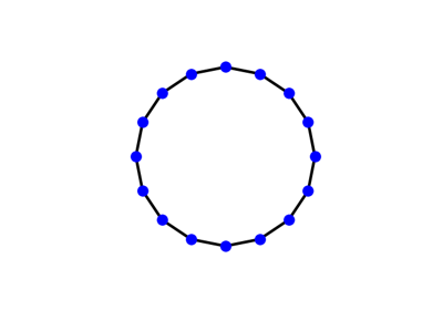
set_peierls_phase takes an arbitrary phase function for a non-uniform field or a different gauge. See examples/magnetic_field/plot_magnetic_field.py for an Aharonov-Bohm ring, where the spectrum is checked to be exactly periodic in the enclosed flux.

Aharonov-Bohm Ring: A Magnetic Field on a Lattice

Spin and spin-orbit coupling#

KSpace(lat, spin=True) gives every site a spin-1/2 degree of freedom (orbitals double: 2*i, 2*i+1 are the up/down components of site i). set_onsite/set_hopping then also accept 2x2 matrices – built from tbkit.kspace.PAULI’s Pauli matrices – for spin-dependent terms:

from tbkit.kspace import PAULI

kmele = KSpace(lat, spin=True)
kmele.set_hopping([{'i': 0, 'j': 1, 'R': (0, 0), 't': 1.},
                          {'i': 0, 'j': 1, 'R': (-1, 0), 't': 1.},
                          {'i': 0, 'j': 1, 'R': (0, -1), 't': 1.}])
# intrinsic SOC, along the three second-neighbor vectors a2, -a1, a1-a2
# (120 degrees apart, as the lattice's C3 symmetry requires)
for R in [(0, 1), (-1, 0), (1, -1)]:
    kmele.set_hopping([{'i': 0, 'j': 0, 'R': R, 't': 1j*lam*PAULI['z']}])
    kmele.set_hopping([{'i': 1, 'j': 1, 'R': R, 't': -1j*lam*PAULI['z']}])

A plain number is still accepted for a spin-independent hopping (expanded to t*PAULI['0']), and onsite values accept a pair (E_up, E_down) for a Zeeman-like splitting.

Topology: Berry curvature and Chern numbers#

For a periodic (KSpace) model, chern_number() gives the Chern number of a group of bands (an isolated band, or several occupied bands below a gap), computed by the gauge-invariant Fukui-Hatsugai-Suzuki lattice method – an integer, for a group of bands with a gap above and below it everywhere in the Brillouin zone:

chern = gra.chern_number(bands=[0], nk=40)    # ~0 for plain graphene (gapless!)

berry_curvature() gives the underlying \(\mathbf{k}\)-resolved curvature (chern_number is just its sum, divided by \(2\pi\)). See examples/topology/plot_haldane_topology.py for the Haldane model – the original Chern insulator – reproducing its topological phase transition (Chern number 1 in one phase, 0 in the other) as a sublattice mass term is tuned.

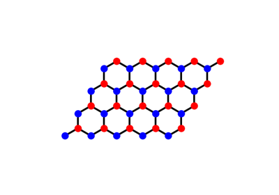
The Haldane Model: Berry Curvature and a Topological Phase Transition

Edge states: cutting a ribbon#

Bulk topology has a physical consequence at an edge. tbkit.kspace.ribbon() cuts a ribbon – periodic along one primitive vector, finite (open boundary, a chosen number of unit cells) along the other – out of any periodic model, keeping its hoppings intact:

from tbkit.kspace import ribbon

list_hop = [{'i': 0, 'j': 1, 'R': (0, 0), 't': 1.},
                  {'i': 0, 'j': 1, 'R': (-1, 0), 't': 1.},
                  {'i': 0, 'j': 1, 'R': (0, -1), 't': 1.}]
rib = ribbon(lat, list_hop, width=30, direction=1)
rib.k_path([(-np.pi,), (np.pi,)], nk=200)
fig = rib.plot_bands()

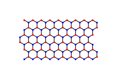
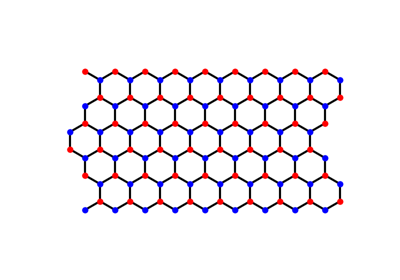
For a zigzag graphene ribbon this reproduces the famous zero-energy edge flat band (examples/tight_binding/plot_zigzag_edge_states.py); cutting a ribbon from the Kane-Mele model above instead shows helical edge states crossing the bulk gap, protected by Kramers’ theorem (examples/topology/plot_edge_states.py). Both are checked numerically.

Zigzag Edge States of Graphene Ribbons

Helical Edge States of the Kane-Mele Ribbon

A ribbon or slab has two surfaces, and its width must beat the decay length of the surface states. surface_spectral_function() avoids both: it gives the spectral function of the outermost cell of a semi-infinite crystal (the iterative surface Green’s function), the tight-binding picture of a photoemission map:

# (001) surface of a 3D model, along a path of k-points of the surface zone
A = ks.surface_spectral_function(path, np.linspace(-2, 2, 201), direction=2)
A_bulk = ks.surface_spectral_function(path, np.linspace(-2, 2, 201), direction=2, bulk=True)

See examples/topology/plot_3d_topological_insulator.py for the surface Dirac cone of a 3D topological insulator.

More topology: Berry phases, Wannier centres, and Z2#

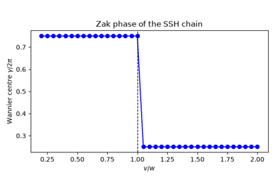
In one dimension (or along one direction of a 2D/3D model), berry_phase() gives the Zak phase of a group of bands – a Wilson loop across the Brillouin zone – and wannier_centers() the positions, in units of the lattice constant, of the corresponding hybrid Wannier functions. For the SSH chain the Wannier centre sits at the middle of the strong bond, inside the cell (0.25 here) or between two cells (0.75):

from tbkit.lattice import Lattice

lat_ssh = Lattice(unit_cell=[{'tag': 'a', 'r0': (0., 0.)}, {'tag': 'b', 'r0': (0.5, 0.)}],
                  prim_vec=[(1., 0.)])
ssh = KSpace(lat_ssh)
ssh.set_hopping([{'i': 0, 'j': 1, 'R': (0,), 't': 0.5},
                        {'i': 1, 'j': 0, 'R': (1,), 't': 1.}])
zak = ssh.berry_phase(0, nk=200)       # -pi/2: Wannier centre at 0.75
centre = ssh.wannier_centers(0, nk=200)

By default the orbital positions inside the cell enter the Bloch phases (positions=True), so the result is a physical polarization; pass positions=False for the periodic-gauge value, which inversion symmetry quantizes to 0 or \(\pi\) (here \(\pi\)). With time-reversal symmetry, wannier_flow() follows the Wannier centres across half the Brillouin zone and z2_invariant() counts how often they wind – the Kane-Mele \(\mathbb{Z}_2\) invariant – while, for an inversion-symmetric model, parity_z2() gets the same number from the Fu-Kane parities at the time-reversal-invariant momenta:

nu = kmele.z2_invariant([0, 1], nk=60, nk_perp=41)

symmetry_error() checks whether a unitary or antiunitary operator is a symmetry of the Bloch Hamiltonian, and tenfold_class() names the Altland-Zirnbauer class; quantum_geometric_tensor() gives the quantum metric (its real part) and Berry curvature (its imaginary part) at one k-point. magnetic_supercell() builds the magnetic Bloch Hamiltonian of a rational flux \(p/q\) per unit cell, whose Chern numbers are the TKNN Hall conductances. Topology survives without translation invariance: on a finite, even disordered, flake get_local_chern_marker() is the Chern number site by site. See examples/topology/.

The Zak Phase: Where the SSH Chain’s Electrons Sit

The Zak Phase: Where the SSH Chain's Electrons Sit

Hall conductivities at any Fermi level#

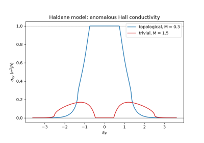
The Chern number is the Hall conductance of a filled group of bands. At any Fermi level – in a gap, inside a band, at finite temperature – hall_conductivity() sums the Berry curvature of the occupied states with the Kubo formula, in units of \(e^2/h\) in 2D (for a 3D model, on a plane, or as the full Hall vector in \(e^2/(h\cdot\mathrm{length})\)). One mesh diagonalization serves a whole array of Fermi energies; for the Haldane model hal of examples/topology/plot_haldane_topology.py:

import numpy as np

e_f = np.linspace(-3., 3., 301)
sigma = hal.hall_conductivity(e_f, nk=120)   # = chern_number in the gap
sigma_t = hal.hall_conductivity(e_f, temperature=0.05, nk=60, refine=4)

In a gap it equals chern_number() (the sign of TKNN; the docstring relates it to the Ohm’s-law tensor). refine resamples the hot spots of the curvature on a finer submesh. spin_hall_conductivity() does the same for the spin current \(\{s_z, v_x\}/2\) of a spinful model, in units of \(e/2\pi\) – 1 in the gap of the Kane-Mele model:

sigma_s = kmele.spin_hall_conductivity(0., nk=60)

For large, disordered samples, tbkit.kpm.hall_conductivity() computes the Kubo-Bastin Hall conductivity in real space, on a torus built by finite_ham() with the velocities of finite_velocity():

import tbkit.kpm as kpm

ham = hal.finite_ham(100, periodic=True, sparse=True)
vx, vy = hal.finite_velocity(100, periodic=True, sparse=True)
area = 100**2 * abs(np.linalg.det(np.array(hal.lat.prim_vec)))
energies, sigma = kpm.hall_conductivity(ham, vx, vy, n_moments=256, area=area)

The same Berry curvature, with other energy weights, gives the orbital magnetization (whose slope in a gap is \(\sigma_{xy}\), the Streda formula), the anomalous Nernst conductivity and the thermal Hall conductivity; axion_angle() follows \(\theta\) of a 3D insulator along a parameter path:

M = hal.orbital_magnetization(e_f, nk=120)
alpha = hal.anomalous_nernst_conductivity(e_f, 0.05, nk=120)
kappa = hal.thermal_hall_conductivity(e_f, 0.05, nk=120)

See examples/hall_effects/, examples/magnetic_field/plot_orbital_magnetization.py and examples/topology/plot_axion_angle.py.

The Anomalous Hall Effect: from the Anomalous Velocity to the Berry Phase

Three dimensions#

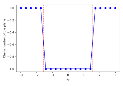
Give the unit cell 3D positions and three primitive vectors and every tool above works in 3D: get_lattice(n1, n2, n3) and Lattice.slab in real space, three-component 'R' in KSpace, and chern_number(..., plane=(0, 1), k_fixed=kz) on a plane of the Brillouin zone – the way to find Weyl points, where it jumps:

cubic = [(1., 0., 0.), (0., 1., 0.), (0., 0., 1.)]
lat = Lattice(unit_cell=[{'tag': 'a', 'r0': (0., 0., 0.)}], prim_vec=cubic)
lat.get_lattice(n1=10, n2=10, n3=10)

ribbon() then cuts a slab (finite along one direction, periodic along the other two). See examples/three_dimensions/.

Weyl Semimetals: Monopoles of Berry Curvature and Fermi Arcs

Several orbitals per site, and Slater-Koster integrals#

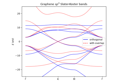
tbkit.slater_koster.sk_kspace() builds a KSpace with several orbitals per site (s, p, d) from Slater-Koster bond integrals, keyed by neighbour order; an optional overlap gives a non-orthogonal basis, and the bands then solve the generalized eigenproblem \(H\psi = ES\psi\):

from tbkit.slater_koster import sk_kspace

orbitals = {'a': ['s', 'px', 'py', 'pz'], 'b': ['s', 'px', 'py', 'pz']}
graphene = sk_kspace(lattices.honeycomb(), orbitals,
                     {1: {'ss_sigma': -6.77, 'sp_sigma': 5.58,
                          'pp_sigma': 5.04, 'pp_pi': -3.03}},
                     onsite={'a': {'s': -8.87}, 'b': {'s': -8.87}})

tbkit.orbital.OrbitalSystem is the real-space counterpart, with spin: Zeeman, atomic and Kane-Mele spin-orbit coupling, Rashba coupling and Peierls phases on multi-orbital flakes. See examples/orbitals/.

The Slater-Koster Method: Graphene’s sigma and pi Bands

The Slater-Koster Method: Graphene's sigma and pi Bands

Large lattices: sparse solvers and the kernel polynomial method#

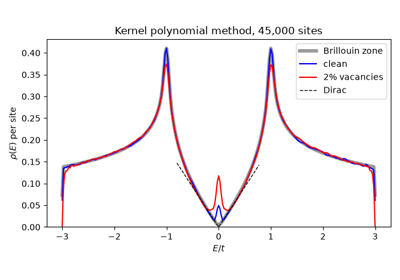
Above System.dense_max sites, System finds neighbours with a k-d tree instead of a dense distance matrix, and get_eig_sparse() finds a few eigenstates near an energy by shift-invert. For spectral quantities of hundreds of thousands of sites, tbkit.kpm expands them in Chebyshev polynomials – density of states, local density of states and the Kubo-Greenwood conductivity – at the cost of a few hundred sparse matrix-vector products:

import tbkit.kpm as kpm

energies, rho = kpm.dos(sys.ham, n_moments=256, n_random=24)

See examples/large_scale/.

The Kernel Polynomial Method: Graphene With Vacancies, 45,000 Sites

Green’s functions, occupations, and transport#

get_green() and get_ldos() give the retarded Green’s function and local density of states; get_fermi_level(), get_occupations and get_charge_density fill the levels with a given number of electrons, at zero or finite temperature (tbkit.occupation). tbkit.transport.Transport attaches semi-infinite leads to a finite device and returns the Landauer transmission, from the scattering matrix of the exact lead modes (smatrix()). The scattering states and their local density of states come from wave_function() and ldos().

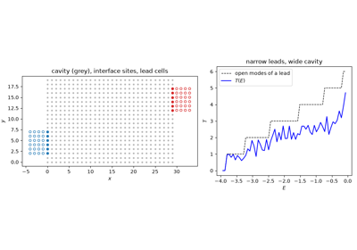
A lead is any 1D KSpace model, for example a strip cut with ribbon(), its orbitals placed in the device’s coordinates. attach_lead() finds the device sites under the lead and couples them with the lead’s own hoppings:

from tbkit.transport import Transport

# strip: a KSpace ribbon, the cross-section of the leads
tr = Transport(sys.ham)
tr.attach_lead(sys, strip, -1)            # continued to -x
tr.attach_lead(sys, strip, 1)             # continued to +x
conductance = tr.transmission(energies)   # in units of e^2/h
s = tr.smatrix(energies[0])               # mode-resolved: s.submatrix(1, 0)

add_lead() attaches a lead by hand: its cell Hamiltonian and coupling (lead_from_kspace() cuts them from a KSpace model), a coupling matrix and the device sites it touches. A device whose edge is ragged relative to the lead (a disc under a strip) is completed with attach_lead(sys, strip, 1, extend=True), which adds the missing lead sites and returns the enlarged Hamiltonian and site positions. See examples/transport/.

Automatic Lead Attachment: Narrow Contacts on a Wide Cavity

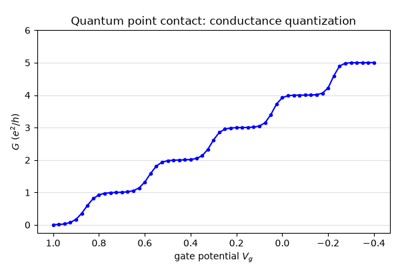
The Landauer Formula: Quantized Conductance of a Point Contact

Interactions and superconductivity#

tbkit.meanfield.hubbard_mean_field() solves the Hubbard model in the unrestricted Hartree-Fock approximation, self-consistently, from any single-particle Hamiltonian:

from tbkit.meanfield import hubbard_mean_field

result = hubbard_mean_field(sys.ham, U=2., n_electrons=sys.lat.sites)
result.magnetization, result.total_spin, result.energy

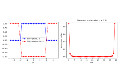
tbkit.bdg builds Bogoliubov-de Gennes Hamiltonians, in real space (bdg_ham with the pairings pairing_bonds/pairing_s_wave) and in reciprocal space (bdg_kspace, a KSpace whose extra orbitals are the holes, so all the topology tools above apply to it). See examples/correlations/ and examples/superconductivity/.

The Kitaev Chain: Majorana Zero Modes

Non-Hermitian bands and Floquet driving#

KSpace.set_hopping(..., hermitian=False) stores a hopping without its conjugate, for non-reciprocal models (the Hatano-Nelson chain); spectral_winding() gives the point-gap winding number that predicts the skin effect, finite_ham() an open or closed finite chain, and gbz() the generalized Brillouin zone.

In two dimensions, bands touch at diabolical points (Hermitian degeneracies, such as graphene’s Dirac points) or at exceptional points, where the eigenvectors coalesce as well. tbkit.exceptional tells them apart. Its functions take a 2D KSpace, or any callable returning a matrix for a point of a parameter plane, and a closed loop (circle(), or polygon vertices):

import tbkit.exceptional as ex

# graphene with a non-Hermitian coupling i*gamma between the sublattices
gra.set_hopping([{'i': 0, 'j': 1, 'R': (0, 0), 't': 0.3j},
                 {'i': 1, 'j': 0, 'R': (0, 0), 't': 0.3j}], hermitian=False)
eps = ex.find_exceptional_points(gra, nk=40)   # positions, charges, orders
eps.total_charge                                # 0: EPs come in pairs
loop = ex.circle(eps.k[0], 0.05)
ex.vorticity(gra, loop)                         # +-1/2 (0 around a Dirac point)
ex.discriminant_winding(gra, loop)              # -+1, no band tracking needed
ex.encircle(gra, loop, n_loops=2).phase         # pi: back after 2 loops, sign flipped
arcs = ex.fermi_arcs(gra, nk=60)                # Re E_+ = Re E_- between the EPs

biorthogonal_chern_number() gives the Chern number of a non-Hermitian band from its left and right eigenvectors (the LR, RL, RR and LL definitions agree) when a real or imaginary line gap isolates it. chern_number() raises a ValueError for a non-Hermitian band without a real line gap. See examples/non_hermitian/plot_exceptional_point*.py and examples/topology/plot_diabolical_points.py.

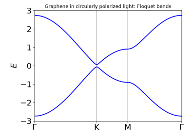
tbkit.floquet handles time-periodic Hamiltonians: the evolution operator over a period, quasienergies, the Floquet Hamiltonian and the Sambe (extended-space) Hamiltonian. tbkit.floquet.FloquetKSpace drives a KSpace with a vector potential \(\mathbf{A}(t)\) and behaves as the static KSpace of its Floquet Hamiltonian – bands, Chern numbers and all:

from tbkit.floquet import FloquetKSpace

omega, a0 = 12., 0.6
light = lambda t: (a0 * np.cos(omega * t), a0 * np.sin(omega * t))
driven = FloquetKSpace(gra, light, 2 * np.pi / omega, n_steps=60)
chern = driven.chern_number(0, nk=16)

The Chern numbers of \(H_F\) do not always count a driven system’s edge states: in anomalous Floquet phases every band has \(C = 0\) while chiral edge states cross every gap. tbkit.floquet.step_drive() builds a piecewise-constant drive from a list of models (KSpace models, ribbons, or System flakes), evolved exactly; winding_number() gives the winding number of Rudner et al. in the gap at epsilon, and edge_state_count() counts the edge states of a driven ribbon:

from tbkit.floquet import step_drive

# models[s]: the KSpace of step s (hopping along one bond direction)
drive = step_drive(models, [T / 5] * 5)
w = drive.winding_number(epsilon=np.pi / T)      # 1 at perfect transfer

See examples/non_hermitian/plot_skin_effect.py and examples/floquet/.

Floquet Engineering: A Chern Insulator From Circularly Polarized Light

Where next#

API – the full API reference, generated from the source docstrings.
examples/ in the repository – runnable scripts for everything above, plus more (kagome, Lieb, propagation, …).
tests/ – every claim above (flat bands, Chern numbers, Kramers degeneracy, flux periodicity, …) is checked against an analytic or independently-computed result somewhere in the test suite; reading them alongside the code they test is a good way to see the underlying physics made concrete.