The Slater-Koster Method: Graphene’s sigma and pi Bands

J. Slater and G. Koster (1954) turned the linear combination of atomic orbitals into a practical band-structure method: the hopping between orbital \(\alpha\) on one atom and \(\beta\) on a neighbour along \(\hat{\mathbf{d}} = (l, m, n)\) follows from a few bond integrals \(V_{ss\sigma}, V_{sp\sigma}, V_{pp\sigma}, V_{pp\pi}, \dots\) through the geometry alone, e.g.

\[E_{s,x} = l\,V_{sp\sigma}\, ,\qquad E_{x,x} = l^2V_{pp\sigma} + (1-l^2)V_{pp\pi}\, ,\]

and they showed how the overlap between orbitals on neighbouring atoms turns the eigenproblem into \(H\psi = ES\psi\).

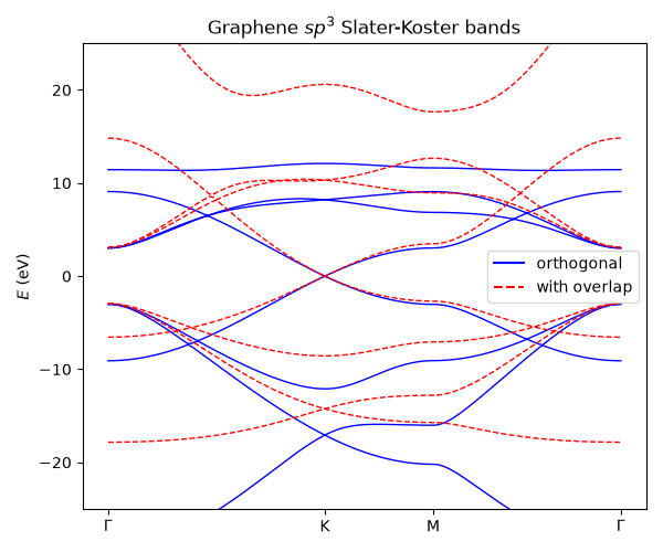
Graphene with the four valence orbitals \(s, p_x, p_y, p_z\) of each carbon (sk_kspace()): the in-plane orbitals hybridize into the \(\sigma\) bands, while \(p_z\) is odd under the mirror of the plane and decouples into the two \(\pi\) bands of Wallace’s model, with \(t = V_{pp\pi}\). With the overlap \(s = S_{pp\pi}\) those become (Saito, Dresselhaus and Dresselhaus)

\[E_\pm(\mathbf{k}) = \frac{\epsilon_p \pm t|f(\mathbf{k})|}{1 \pm s|f(\mathbf{k})|}\, ,\]

no longer symmetric about \(\epsilon_p\).

import numpy as np
import matplotlib.pyplot as plt

import tbkit.lattices as lattices
from tbkit.kspace import reciprocal_vectors
from tbkit.orbital import OrbitalSystem
from tbkit.slater_koster import sk_kspace
from tbkit.plot import Plot
from tbkit.system import System

# eV; energies relative to the 2p level (Saito, Dresselhaus and Dresselhaus)
orbitals = {'a': ['s', 'px', 'py', 'pz'], 'b': ['s', 'px', 'py', 'pz']}
onsite = {'a': {'s': -8.87}, 'b': {'s': -8.87}}
hopping = {'ss_sigma': -6.77, 'sp_sigma': 5.58, 'pp_sigma': 5.04, 'pp_pi': -3.03}
overlap = {'ss_sigma': 0.212, 'sp_sigma': -0.102, 'pp_sigma': -0.146, 'pp_pi': 0.129}

lat = lattices.honeycomb()
graphene = sk_kspace(lat, orbitals, {1: hopping}, onsite=onsite)
graphene_s = sk_kspace(lat, orbitals, {1: hopping}, onsite=onsite, overlap={1: overlap})
pz = [n for n, (_, o) in enumerate(graphene.sk_orbitals) if o == 'pz']

b1, b2 = (np.array(v) for v in reciprocal_vectors(lat.prim_vec))
Gamma, K, M = np.zeros(2), (b1 - b2) / 3, b1 / 2
t, s = hopping['pp_pi'], overlap['pp_pi']


def f_abs(k):
    a = np.array(lat.prim_vec)
    return abs(sum(np.exp(1j * k @ (n1 * a[0] + n2 * a[1])) for n1, n2 in [(0, 0), (-1, 0), (0, -1)]))

The lattice

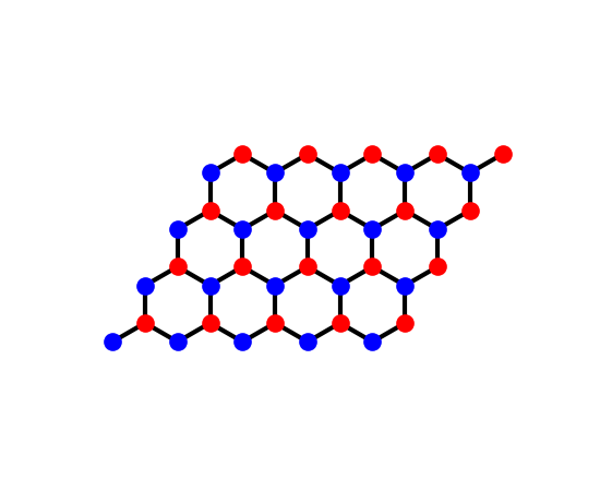
Graphene’s honeycomb lattice, sublattices a and b in two colours, each atom carrying the four orbitals \(s, p_x, p_y, p_z\) and bonded to its three nearest neighbours by the Slater-Koster integrals above.

patch = lattices.honeycomb()
patch.get_lattice(n1=5, n2=4)
vis = System(patch)
vis.set_hopping([{'n': 1, 't': 1.}])
fig_lat = Plot(vis).lattice(plt_hop=True, ms=12, figsize=(5.5, 4.5))

pz decouples: the pi bands are Wallace’s

for k in (Gamma, K, M, 0.3*b1 + 0.1*b2):
    ham = graphene.get_ham(k)
    others = [n for n in range(8) if n not in pz]
    assert np.allclose(ham[np.ix_(pz, others)], 0.)
    pi = np.linalg.eigvalsh(ham[np.ix_(pz, pz)])
    assert np.allclose(pi, [-abs(t) * f_abs(k), abs(t) * f_abs(k)])
# the Dirac point: the two pi bands meet at E = eps_p = 0 at K
assert np.allclose(np.linalg.eigvalsh(graphene.get_ham(K))[3:5], 0.)
print('pz decouples; pi bands = +-|V_pp_pi||f(k)|, touching at K.')

pz decouples; pi bands = +-|V_pp_pi||f(k)|, touching at K.

The overlap breaks the electron-hole symmetry of the pi bands

for k in (Gamma, M, 0.3*b1 + 0.1*b2):
    en = graphene_s.get_bands([k]).ravel()
    exact = [(-t*f_abs(k)) / (1 - s*f_abs(k)), (t*f_abs(k)) / (1 + s*f_abs(k))]
    for e in exact:
        assert np.min(np.abs(en - e)) < 1e-9
print('At Gamma, the pi bands sit at {:.2f} and {:.2f} eV: asymmetric about 0.'
          .format(t*3 / (1 + 3*s), -t*3 / (1 - 3*s)))

At Gamma, the pi bands sit at -6.55 and 14.83 eV: asymmetric about 0.

The same model on a finite flake

OrbitalSystem builds the same Slater-Koster blocks bond by bond in real space: its spectrum equals that of the Bloch model cut to the same open parallelogram.

flake = lattices.honeycomb()
flake.get_lattice(5, 4)
sys = OrbitalSystem(flake, orbitals=orbitals)
sys.set_onsite(onsite)
sys.set_slater_koster(1, hopping)
sys.get_ham()
sys.get_eig()
assert np.allclose(sys.en, np.linalg.eigvalsh(graphene.finite_ham((5, 4))))

fig, ax = plt.subplots(figsize=(6, 5))
for model, style, label in ((graphene, 'b', 'orthogonal'), (graphene_s, 'r--', 'with overlap')):
    dist, en = model.k_path([Gamma, K, M, Gamma], nk=60)
    ax.plot(dist, en, style, lw=1)
    ax.plot([], [], style, label=label)
ax.set_xticks(graphene_s.nodes)
ax.set_xticklabels([r'$\Gamma$', 'K', 'M', r'$\Gamma$'])
ax.set_ylabel('$E$ (eV)')
ax.set_ylim(-25, 25)
ax.legend()
ax.set_title(r'Graphene $sp^3$ Slater-Koster bands')
fig.set_layout_engine('tight')