The Berry-Phase Anomalous Nernst Effect

A temperature gradient drives a transverse charge current in a ferromagnet, with no magnetic field: the anomalous Nernst effect, \(j_x = \alpha_{xy}(-\partial_yT)\). Xiao, Yao, Fang and Niu (2006) showed that its intrinsic part is the Berry curvature again, weighted this time by the entropy of each state,

\[\alpha_{xy} = \frac{ek_B}{h}\,\frac{1}{2\pi}\int_{BZ}d^2k\sum_ns_n\,\Omega_n\, , \qquad s = -f\ln f-(1-f)\ln(1-f)\, .\]

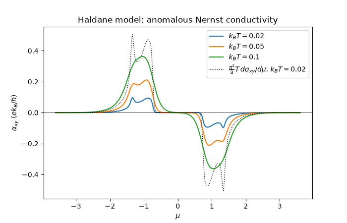
The orbital magnetization makes it work: a statistical gradient drives no current through a uniform \(\mathbf{M}\), but a thermal gradient does through its edge-current part. Only states within a few \(k_BT\) of \(\mu\) carry entropy, so \(\alpha_{xy}\) vanishes in a gap, peaks near band edges where the curvature is large, and obeys the Mott relation exactly,

\[\alpha_{xy}(\mu, T) = \frac{1}{eT}\int dE\,(E-\mu)\left(-\frac{\partial f}{\partial E}\right)\sigma_{xy}(E) \;\xrightarrow{T\to0}\; \frac{\pi^2k_B^2T}{3e}\,\frac{d\sigma_{xy}}{d\mu}\, .\]

anomalous_nernst_conductivity() evaluates it for the Haldane model below.

import numpy as np
import matplotlib.pyplot as plt
from scipy.integrate import trapezoid

import tbkit.lattices as lattices
from tbkit.bridges import finite_system
from tbkit.kspace import KSpace
from tbkit.plot import Plot


def haldane(M, t2=0.2):
    '''Haldane model: nearest-neighbour t = 1, i t2 on the second neighbours, mass +-M.'''
    hal = KSpace(lattices.honeycomb())
    hal.set_hopping([{'i': 0, 'j': 1, 'R': R, 't': 1.} for R in [(0, 0), (-1, 0), (0, -1)]])
    for R in [(0, 1), (-1, 0), (1, -1)]:
        hal.set_hopping([{'i': 0, 'j': 0, 'R': R, 't': 1j*t2}, {'i': 1, 'j': 1, 'R': R, 't': -1j*t2}])
    hal.set_onsite({'a': M, 'b': -M})
    return hal


hal = haldane(0.3)

The lattice

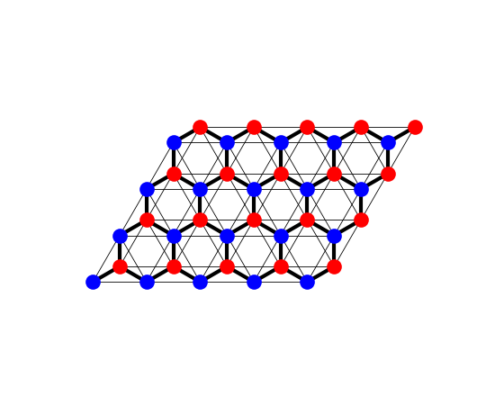
The Haldane model on a patch of \(5\times4\) cells (finite_system()), each bond drawn with a width proportional to its amplitude: the honeycomb lattice’s two sublattices (‘a’ and ‘b’, in two colours), the nearest-neighbour hopping \(t\) (thick) and the complex second-neighbour hoppings \(\pm it_2\) within each sublattice (thin), which break time-reversal symmetry.

fig_lat = Plot(finite_system(haldane(0.3), (5, 4))).lattice(plt_hop=True, ms=12, figsize=(5.5, 4.5))

The Nernst conductivity across the spectrum

At three temperatures. It vanishes in the gap at low temperature (no entropy there), and in empty or full bands.

mu = np.linspace(-3.6, 3.6, 361)
temps = (0.02, 0.05, 0.1)
alpha = {T: hal.anomalous_nernst_conductivity(mu, T, nk=120) for T in temps}

gap = (np.abs(mu) < 0.2)
print('T = 0.02: |alpha| in the gap below {:.1e}'.format(np.max(np.abs(alpha[0.02][gap]))))
assert np.max(np.abs(alpha[0.02][gap])) < 1e-6
# empty and full bands carry no entropy
assert np.max(np.abs(hal.anomalous_nernst_conductivity(np.array([-6., 6.]), 0.1, nk=60))) < 1e-10

T = 0.02: |alpha| in the gap below 6.0e-13

The Mott relation

The same numbers from the \(T = 0\) Hall conductivity \(\sigma_{xy}(E)\) on a fine energy grid, integrated against the thermal window \((E-\mu)(-\partial f/\partial E)/T\). At low temperature, the Sommerfeld expansion leaves \(\frac{\pi^2}{3}T\,d\sigma_{xy}/d\mu\): within 4% of the peak at \(k_BT = 0.02\), inside the lower band.

e = np.linspace(-4., 4., 4001)
sigma = hal.hall_conductivity(e, nk=120)
for T in temps:
    x = np.abs(e[:, None] - mu[None, :]) / T
    window = np.exp(-x) / (1 + np.exp(-x)) ** 2 / T
    mott = trapezoid((e[:, None] - mu) * window * sigma[:, None], e, axis=0) / T
    err = np.max(np.abs(alpha[T] - mott))
    print('T = {}: max |alpha - Mott| = {:.1e}'.format(T, err))
    assert err < 5e-4

T = 0.02
deriv = np.gradient(hal.hall_conductivity(mu, T, nk=120), mu)
band = (mu > -2.5) & (mu < -1.0)  # where sigma_xy(mu) is smooth
low_t = np.max(np.abs(alpha[T][band] - np.pi ** 2 / 3 * T * deriv[band]))
print('T = 0.02: max |alpha - pi^2/3 T dsigma/dmu| in the band = {:.1e}'.format(low_t))
assert low_t < 0.04 * np.max(np.abs(alpha[T][band]))

fig, ax = plt.subplots(figsize=(7, 4.5))
for T in temps:
    ax.plot(mu, alpha[T], label='$k_BT = {}$'.format(T))
ax.plot(mu, np.pi ** 2 / 3 * T * deriv, 'k:', lw=1,
        label=r'$\frac{\pi^2}{3}T\,d\sigma_{xy}/d\mu$, $k_BT = 0.02$')
ax.axhline(0., color='k', lw=0.5)
ax.set_xlabel(r'$\mu$')
ax.set_ylabel(r'$\alpha_{xy}$ ($ek_B/h$)')
ax.set_title('Haldane model: anomalous Nernst conductivity')
ax.legend()

T = 0.02: max |alpha - Mott| = 1.2e-04
T = 0.05: max |alpha - Mott| = 4.8e-05
T = 0.1: max |alpha - Mott| = 4.0e-05
T = 0.02: max |alpha - pi^2/3 T dsigma/dmu| in the band = 3.3e-03

<matplotlib.legend.Legend object at 0x10f25a660>