The Axion Angle and the Topological Magnetoelectric Effect

An insulator responds to an electric field with a magnetization and to a magnetic field with a polarization. Part of that response is a single number \(\theta\), entering the electromagnetic action as the axion term of Wilczek (1987), \(\frac{\theta e^2}{2\pi h}\int\mathbf{E}\cdot\mathbf{B}\): the polarization \(\mathbf{P} = \frac{\theta}{2\pi}\frac{e^2}{h}\mathbf{B}\). Qi, Hughes and Zhang (2008) and Essin, Moore and Vanderbilt (2009) showed that for Bloch electrons \(\theta\) is the Chern-Simons integral of the Berry connection of the occupied bands. It is defined modulo \(2\pi\) (a surface can always gain a quantum Hall layer), and time reversal or inversion force \(\theta = 0\) or \(\pi\): \(\pi\) is the strong 3D topological insulator.

Along a gapped path of Hamiltonians, \(\theta\) changes by the integral of the second Chern form, a gauge-invariant quantity, and over a closed cycle by \(2\pi C_2\) – the 3D analogue of the Thouless pump, which pumps a quantum Hall layer instead of a charge.

axion_angle() integrates it for a lattice Dirac model with four bands,

\[H = \sum_i\sin k_i\,\Gamma_i + \left(m + \sum_i\cos k_i + \cos\phi\right)\Gamma_0 + \sin\phi\,\Gamma_4\, ,\]

whose \(\Gamma_4\) term breaks time reversal and inversion except at \(\phi = 0, \pi\). For \(m = 3\) it is trivial at \(\phi = 0\) (Dirac mass 4) and a strong topological insulator at \(\phi = \pi\) (mass 2), and the gap never closes along the way.

import numpy as np
import matplotlib.pyplot as plt
from mpl_toolkits.mplot3d.art3d import Line3DCollection

from tbkit.kspace import KSpace, PAULI
from tbkit.lattice import Lattice
from tbkit.system import System


def axion_model(m):
    '''The Dirac model above; phi is a parameter of its value functions.'''
    lat = Lattice(unit_cell=[{'tag': t, 'r0': (0., 0., 0.)} for t in 'abcd'],
                         prim_vec=[(1., 0., 0.), (0., 1., 0.), (0., 0., 1.)])
    ks = KSpace(lat)
    g0 = np.kron(PAULI['x'], PAULI['0'])  # Gamma_0; Gamma_i = sz x s_i, Gamma_4 = sy x 1
    hop = []
    for ax, s in enumerate('xyz'):
        block = np.kron(PAULI['z'], PAULI[s]) / 2j + g0 / 2  # sin k Gamma_i + cos k Gamma_0
        hop += [{'i': i, 'j': j, 'R': tuple(int(a == ax) for a in range(3)), 't': complex(block[i, j])}
                     for i in range(4) for j in range(4) if block[i, j] != 0]
    ks.set_hopping(hop)
    # (m + cos phi) Gamma_0 + sin phi Gamma_4, on the orbital pairs (0, 2) and (1, 3)
    ks.set_hopping([{'i': o, 'j': o + 2, 'R': (0, 0, 0), 't': lambda si, sj, phi: m + np.exp(-1j * phi)}
                             for o in (0, 1)])
    ks.set_params(phi=0.)
    return ks

The lattice

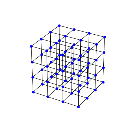
The simple cubic lattice, here \(4\times4\times4\) sites, with its nearest-neighbour bonds. Each site holds the four orbitals of the Dirac model, and every bond carries a \(4\times4\) hopping matrix that couples them (not drawn).

lat_vis = Lattice(unit_cell=[{'tag': 'a', 'r0': (0., 0., 0.)}], prim_vec=[(1., 0., 0.), (0., 1., 0.), (0., 0., 1.)])
lat_vis.get_lattice(4, 4, 4)
vis = System(lat_vis)
vis.set_hopping([{'n': 1, 't': 1.}])
pos = np.column_stack([lat_vis.coor[f] for f in 'xyz'])
bonds = np.stack([pos[vis.hop['i'].astype(int)], pos[vis.hop['j'].astype(int)]], axis=1)
fig_lat = plt.figure(figsize=(4.5, 4.5))
ax_lat = fig_lat.add_subplot(projection='3d')
ax_lat.add_collection3d(Line3DCollection(bonds, colors='k', linewidths=1))
ax_lat.scatter(*pos.T, s=30, c='b', depthshade=False)
ax_lat.set_aspect('equal')
ax_lat.set_axis_off()

Theta along the pumping cycle

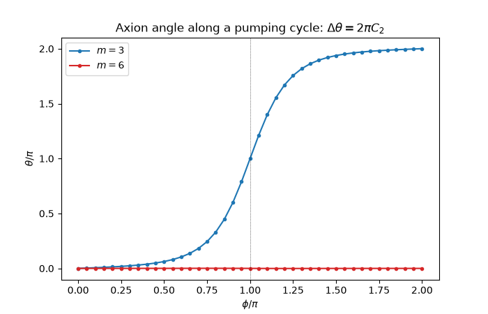
Starting from \(\theta = 0\) at the trivial point, the second Chern form brings \(\theta\) to \(\pi\) exactly where time reversal is restored, and to \(2\pi\) at the end of the cycle (\(C_2 = 1\)). A model deep in the trivial phase (\(m = 6\)) pumps nothing: its \(\theta\) stays within \(10^{-3}\pi\) of 0 along the whole cycle.

phi = np.linspace(0., 2 * np.pi, 41)
theta = {m: axion_model(m).axion_angle([0, 1], 'phi', phi, nk=16) for m in (3., 6.)}

half = theta[3.][20] / np.pi
print('m = 3: theta(pi) = {:.5f} pi, theta(2 pi) = {:.5f} pi'.format(half, theta[3.][-1] / np.pi))
assert abs(half - 1.) < 1e-3 and abs(theta[3.][-1] / np.pi - 2.) < 1e-3
print('m = 6: theta(pi) = {:.1e}, theta(2 pi) = {:.1e}'.format(theta[6.][20], theta[6.][-1]))
assert np.max(np.abs(theta[6.])) < 1e-3 * np.pi

m = 3: theta(pi) = 1.00016 pi, theta(2 pi) = 2.00033 pi
m = 6: theta(pi) = -4.7e-08, theta(2 pi) = -9.4e-08

The end points agree with the strong Z2 index (Fu-Kane-Mele), computed independently from Wilson loops at the time-reversal symmetric points.

for m in (3., 6.):
    ks = axion_model(m)
    for p in (0., np.pi):
        ks.set_params(phi=p)
        nu0 = ks.z2_indices_3d([0, 1], nk=10)[0]
        k = int(round(p / (phi[1] - phi[0])))
        print('m = {}, phi = {:.2f}: nu_0 = {}, theta = {:.4f} pi'.format(m, p, nu0, theta[m][k] / np.pi))
        assert abs(theta[m][k] / np.pi - nu0) < 1e-3

fig, ax = plt.subplots(figsize=(7, 4.5))
for m, color in ((3., 'C0'), (6., 'C3')):
    ax.plot(phi / np.pi, theta[m] / np.pi, 'o-', ms=3, color=color, label='$m = {:g}$'.format(m))
ax.set_xlabel(r'$\phi/\pi$')
ax.set_ylabel(r'$\theta/\pi$')
ax.set_yticks([0, 0.5, 1, 1.5, 2])
ax.axvline(1., color='k', lw=0.5, ls=':')
ax.set_title(r'Axion angle along a pumping cycle: $\Delta\theta = 2\pi C_2$')
ax.legend()

m = 3.0, phi = 0.00: nu_0 = 0, theta = 0.0000 pi
m = 3.0, phi = 3.14: nu_0 = 1, theta = 1.0002 pi
m = 6.0, phi = 0.00: nu_0 = 0, theta = 0.0000 pi
m = 6.0, phi = 3.14: nu_0 = 0, theta = -0.0000 pi

<matplotlib.legend.Legend object at 0x115b774d0>