The Kernel Polynomial Method: Graphene With Vacancies, 45,000 Sites

Diagonalizing \(N\) sites costs \(N^3\) operations and \(N^2\) memory: a few thousand sites at most. The kernel polynomial method (Silver and Roder, 1994; reviewed by Weisse, Wellein, Alvermann and Fehske, Rev. Mod. Phys. 78, 275 (2006)) never diagonalizes. It expands the spectral density in Chebyshev polynomials of the rescaled Hamiltonian,

\[\rho(E) = \frac{1}{\pi\sqrt{1-\epsilon^2}}\Big[\mu_0 + 2\sum_{m\ge1} g_m\,\mu_m T_m(\epsilon)\Big]\, ,\qquad \mu_m = \mathrm{Tr}\,T_m(\tilde H)\, ,\]

computing each moment with one sparse matrix-vector product (the Chebyshev recursion) and the trace with a few random vectors; the Jackson kernel \(g_m\) removes the Gibbs oscillations of the truncated series. The cost is linear in \(N\).

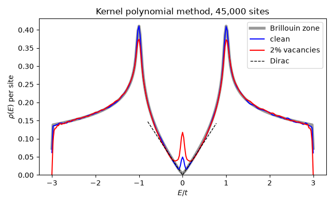
Here: the density of states of a graphene sheet of 45,000 sites (tbkit.kpm), clean – the linear Dirac density of states and the van Hove peaks at \(E = \pm t\) – and with 2% of the sites removed, which piles up states at \(E = 0\) (vacancy-bound zero modes).

import numpy as np
import matplotlib.pyplot as plt
from scipy.integrate import trapezoid

import tbkit.kpm as kpm
import tbkit.lattices as lattices
from tbkit.kspace import KSpace
from tbkit.plot import Plot
from tbkit.system import System

t = 1.
n = 150  # 150 x 150 unit cells: 45,000 sites


def graphene(vacancies=0., seed=0):
    lat = lattices.honeycomb()
    lat.get_lattice(n, n)
    if vacancies:
        rng = np.random.default_rng(seed)
        lat.remove_sites(sorted(rng.choice(lat.sites, int(vacancies * lat.sites), replace=False).tolist()))
    sys = System(lat)  # beyond System.dense_max: neighbours from a k-d tree
    sys.set_hopping([{'n': 1, 't': t}])
    sys.get_ham()
    return sys

The lattice

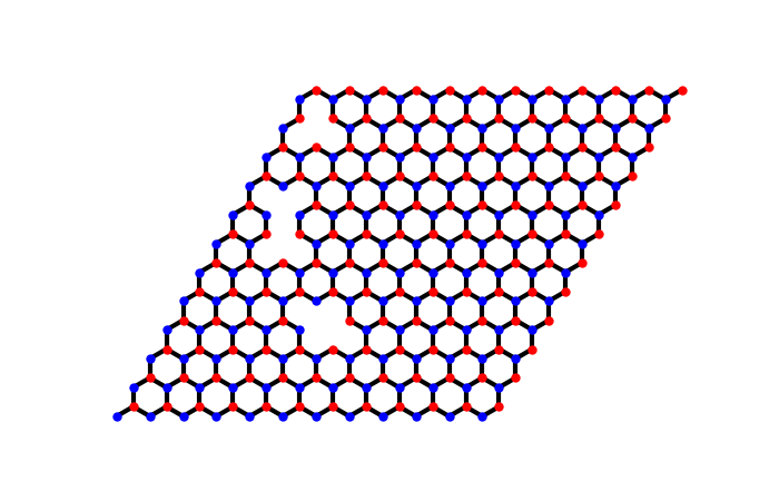
The honeycomb lattice – sublattices ‘a’ and ‘b’ in two colours – with 2% of its sites removed at random, here on a \(12\times12\) corner of the flake. The flake used below is 150 cells on a side.

lat_vis = lattices.honeycomb()
lat_vis.get_lattice(12, 12)
rng_vis = np.random.default_rng(0)
lat_vis.remove_sites(sorted(rng_vis.choice(lat_vis.sites, int(0.02 * lat_vis.sites),
                                                    replace=False).tolist()))
vis = System(lat_vis)
vis.set_hopping([{'n': 1, 't': t}])
fig_lat = Plot(vis).lattice(plt_hop=True, ms=6, figsize=(7, 4.5))

The density of states of the clean flake and of one with 2% vacancies, by the kernel polynomial method:

e_grid = np.linspace(-3., 3., 241)
clean = graphene()
_, rho_clean = kpm.dos(clean.ham, n_moments=256, n_random=24, e_grid=e_grid, seed=1)
rho_clean = rho_clean / clean.lat.sites
dirty = graphene(vacancies=0.02)
_, rho_dirty = kpm.dos(dirty.ham, n_moments=256, n_random=24, e_grid=e_grid, seed=1)
rho_dirty = rho_dirty / dirty.lat.sites
print('{} sites (clean), {} sites (2% vacancies).'.format(clean.lat.sites, dirty.lat.sites))

45000 sites (clean), 44100 sites (2% vacancies).

Against the Brillouin zone, and the Dirac law

The reference: the bands of the infinite sheet on a 400 x 400 k-mesh (KSpace), broadened by the same Jackson-damped Chebyshev series (dos_from_levels()). Near the Dirac point, per site, \(\rho(E) = \frac{A_c}{2\pi v_F^2}|E| = \frac{|E|}{\sqrt3\,\pi t^2}\) (\(A_c = 3\sqrt3/2\) the cell area, \(v_F = 3t/2\)).

bloch = KSpace(lattices.honeycomb())
bloch.set_hopping([{'i': 0, 'j': 1, 'R': R, 't': t} for R in [(0, 0), (-1, 0), (0, -1)]])
bands = bloch.mesh_bands(400)
rho_bz = kpm.dos_from_levels(bands, 256, kpm.spectral_bounds(clean.ham), e_grid) / bands.size
window = (np.abs(e_grid) > 0.6) & (np.abs(e_grid) < 2.7)
deviation = np.max(np.abs(rho_clean[window] / rho_bz[window] - 1.))
print('KPM vs Brillouin-zone DOS, 0.6 < |E| < 2.7: largest deviation {:.1%}'.format(deviation))
assert deviation < 0.03
# closer to the Dirac point (|E| < 0.5) the finite flake's quantized
# momenta (and its edges) start to show, at the level of a few percent
for e in (0.3, 0.4):
    kpm_value = np.interp(e, e_grid, rho_clean)
    dirac = e / (np.sqrt(3) * np.pi * t**2)
    print('rho({}) = {:.4f}, Dirac law: {:.4f}'.format(e, kpm_value, dirac))
    assert abs(kpm_value / dirac - 1.) < 0.08
# van Hove singularities at |E| = t
peak = e_grid[np.argmax(rho_clean * (e_grid > 0))]
print('van Hove peak at E = {:.3f}'.format(peak))
assert abs(peak - t) < 0.05
assert np.isclose(trapezoid(rho_clean, e_grid), 1., atol=0.01)

KPM vs Brillouin-zone DOS, 0.6 < |E| < 2.7: largest deviation 2.2%
rho(0.3) = 0.0545, Dirac law: 0.0551
rho(0.4) = 0.0744, Dirac law: 0.0735
van Hove peak at E = 1.000

Vacancies: states at zero energy

Each vacancy binds a state at \(E = 0\) on the other sublattice: 2% of vacancies more than double the (broadened) density of states there.

print('rho(0): clean {:.4f}, with vacancies {:.4f}.'.format(rho_clean[120], rho_dirty[120]))
assert rho_dirty[120] > 2 * rho_clean[120]

fig, ax = plt.subplots(figsize=(6.5, 4))
ax.plot(e_grid, rho_bz, color='0.6', lw=4, label='Brillouin zone')
ax.plot(e_grid, rho_clean, 'b', label='clean')
ax.plot(e_grid, rho_dirty, 'r', label='2% vacancies')
ax.plot(e_grid[np.abs(e_grid) < 0.8], np.abs(e_grid[np.abs(e_grid) < 0.8]) / (np.sqrt(3)*np.pi),
           'k--', lw=1, label='Dirac')
ax.set_xlabel('$E/t$')
ax.set_ylabel(r'$\rho(E)$ per site')
ax.set_ylim(0, None)
ax.legend()
ax.set_title('Kernel polynomial method, 45,000 sites')
fig.set_layout_engine('tight')

rho(0): clean 0.0495, with vacancies 0.1176.