Saving and Reloading Models: a Kane-Mele Model on Disk

tbkit.io.save_model() writes a Lattice, System or KSpace to a versioned .npz archive – plain NumPy arrays, no pickle – and tbkit.io.load_model() reads it back. Onsite terms, hoppings, overlaps and spin are stored in binary, so the reloaded model reproduces the Hamiltonians bit for bit.

The example saves a spinful Kane-Mele model (a KSpace with 2x2 spin blocks) and a disordered real-space flake (a System, whose random hoppings could not be regenerated), reloads both, and checks that every matrix and spectrum is identical.

import os
import tempfile

import numpy as np
import matplotlib.pyplot as plt

from tbkit import lattices
from tbkit.io import save_model, load_model
from tbkit.kspace import KSpace, PAULI
from tbkit.plot import Plot
from tbkit.system import System

A spinful Bloch model

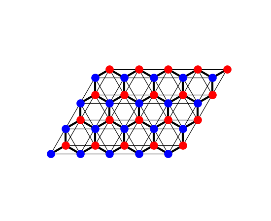
Graphene with the intrinsic spin-orbit coupling of Kane and Mele: \(i\lambda\nu_{ij}\sigma_z\) on second neighbours (\(\nu = +1\) for the sublattice-a bonds at 0, 120 and 240 degrees, conjugate for the stored 60-degree bond, the opposite on sublattice b).

t, lam = 1., 0.06
so, so_c = 1j * lam * PAULI['z'], -1j * lam * PAULI['z']
km = KSpace(lattices.honeycomb(), spin=True)
km.set_hopping([{'n': 1, 't': t},
                        {'n': 2, 'tag': 'aa', 'ang': 0., 't': so}, {'n': 2, 'tag': 'aa', 'ang': 60., 't': so_c},
                        {'n': 2, 'tag': 'aa', 'ang': 120., 't': so},
                        {'n': 2, 'tag': 'bb', 'ang': 0., 't': so_c}, {'n': 2, 'tag': 'bb', 'ang': 60., 't': so},
                        {'n': 2, 'tag': 'bb', 'ang': 120., 't': so_c}])

Its bonds on a patch of the honeycomb lattice (sublattices a and b in two colours): the nearest-neighbour hopping \(t\) (thick) and the second-neighbour spin-orbit bonds (thin, not to scale; their spin matrices \(\pm i\lambda\sigma_z\) are not drawn).

patch = lattices.honeycomb()
patch.get_lattice(n1=5, n2=4)
vis = System(patch)
vis.set_hopping([{'n': 1, 't': t}, {'n': 2, 't': 5 * lam}])
fig_lat = Plot(vis).lattice(plt_hop=True, ms=12, figsize=(5.5, 4.5))

A disordered flake

lat = lattices.honeycomb()
lat.get_lattice(10, 10)
flake = System(lat)
flake.set_hopping([{'n': 1, 't': t}])
flake.set_onsite({'a': 0., 'b': 0.})
flake.set_onsite_dis(0.5)
flake.get_ham()
flake.get_eig()

Save, reload, compare

with tempfile.TemporaryDirectory() as tmp:
    km_path = save_model(km, os.path.join(tmp, 'kane_mele'))
    flake_path = save_model(flake, os.path.join(tmp, 'flake.npz'))
    print('wrote', os.path.basename(km_path), 'and', os.path.basename(flake_path))
    with np.load(km_path) as archive:
        print('archive entries:', sorted(archive.files))
    km2 = load_model(km_path)
    flake2 = load_model(flake_path)

rng = np.random.default_rng(0)
for k in rng.uniform(-4., 4., (50, 2)):
    assert np.array_equal(km2.get_ham(k), km.get_ham(k))
flake2.get_ham()
flake2.get_eig()
assert np.array_equal(flake2.ham.toarray(), flake.ham.toarray())
assert np.array_equal(flake2.en, flake.en)

wrote kane_mele.npz and flake.npz
archive entries: ['coor', 'format', 'hop_R', 'hop_i', 'hop_j', 'hop_t', 'kind', 'n_cells', 'nonreciprocal', 'onsite', 'onsite_offdiag', 'ovl_R', 'ovl_i', 'ovl_j', 'ovl_t', 'prim_vec', 'spin', 'tbkit_version', 'uc_r0', 'uc_tag', 'version']

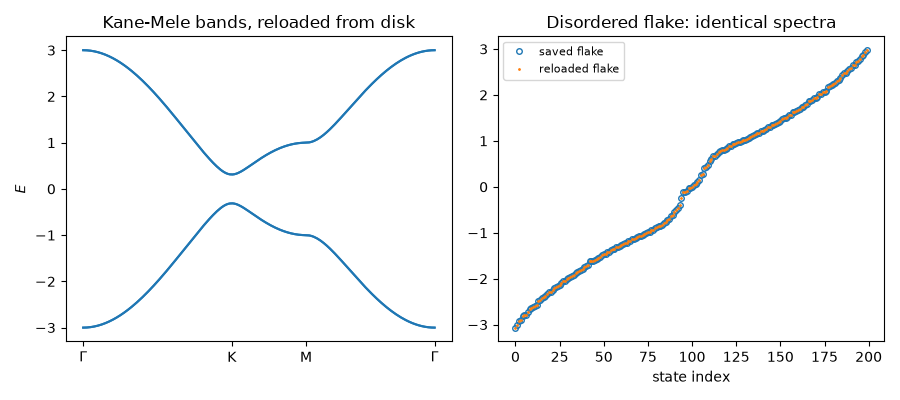
The reloaded Kane-Mele model is still a quantum spin Hall insulator: a gap \(6\sqrt{3}\lambda\) at K and a nontrivial \(\mathbb{Z}_2\) invariant.

b1, b2 = np.array(km2.rec_vec)
K = (b1 - b2) / 3
en_K = km2.get_bands(K)[0]
gap = en_K[2] - en_K[1]
z2 = km2.z2_invariant(bands=[0, 1], nk=24)
print('gap at K = {:.6f} (6 sqrt(3) lambda = {:.6f}), Z2 = {}'.format(gap, 6 * np.sqrt(3) * lam, z2))
assert abs(gap - 6 * np.sqrt(3) * lam) < 1e-12
assert z2 == 1

gap at K = 0.623538 (6 sqrt(3) lambda = 0.623538), Z2 = 1

Bands of the reloaded model, and spectrum of the reloaded flake.

Gamma, M = np.zeros(2), b1 / 2
dist, en = km2.k_path([Gamma, K, M, Gamma], nk=80)
fig, (ax1, ax2) = plt.subplots(1, 2, figsize=(9, 4))
ax1.plot(dist, en, color='C0')
ax1.set_xticks(km2.nodes)
ax1.set_xticklabels([r'$\Gamma$', 'K', 'M', r'$\Gamma$'])
ax1.set_ylabel('$E$')
ax1.set_title('Kane-Mele bands, reloaded from disk')
ax2.plot(flake.en, 'o', ms=4, mfc='none', label='saved flake')
ax2.plot(flake2.en, '.', ms=2, label='reloaded flake')
ax2.set_xlabel('state index')
ax2.set_title('Disordered flake: identical spectra')
ax2.legend(fontsize=8)
fig.tight_layout()
plt.show()