Helical Edge States of the Kane-Mele Ribbon

Cutting a periodic 2D model into a ribbon (periodic in one direction, finite/open in the other – see tbkit.kspace.ribbon()) is the standard way to see edge physics in a tight-binding band structure. Adding Kane-Mele intrinsic spin-orbit coupling to graphene (see The Haldane Model: Berry Curvature and a Topological Phase Transition for the closely related Haldane model) opens a bulk gap and produces helical edge states: gapless, spin-momentum-locked modes that cross the bulk gap, one Kramers pair per edge. This is the original model of a 2D (Z2) topological insulator. Without spin-orbit coupling, the same zigzag ribbon has a flat band of edge states at E=0 instead (see Zigzag Edge States of Graphene Ribbons).

import numpy as np
import matplotlib.pyplot as plt

from tbkit.lattice import Lattice
from tbkit.kspace import ribbon, PAULI
from tbkit.plot import Plot
from tbkit.system import System


DX, DY = 0.5 * 3 ** 0.5, 0.5
unit_cell = [{'tag': 'a', 'r0': (0., 0.)}, {'tag': 'b', 'r0': (DX, DY)}]
prim_vec = [(2*DX, 0.), (DX, 1.5)]
lat = Lattice(unit_cell=unit_cell, prim_vec=prim_vec)
t1 = 1.
graphene_hop = [{'i': 0, 'j': 1, 'R': (0, 0), 't': t1},
                        {'i': 0, 'j': 1, 'R': (-1, 0), 't': t1},
                        {'i': 0, 'j': 1, 'R': (0, -1), 't': t1}]
width = 30

The lattice

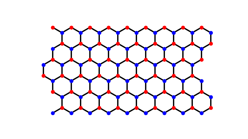
The honeycomb lattice of the ribbons below, sublattices ‘a’ and ‘b’ in two colours, with its nearest-neighbour bonds, on a \(10\times6\)-cell patch (the ribbons are 30 cells wide). The spin-orbit terms are second-neighbour hoppings within each sublattice, not drawn.

patch = Lattice(unit_cell=unit_cell, prim_vec=prim_vec)
patch.get_lattice(n1=10, n2=6)
vis = System(patch)
vis.set_hopping([{'n': 1, 't': t1}])
fig_lat = Plot(vis).lattice(plt_hop=True, ms=8, figsize=(8, 4))

Kane-Mele ribbon: helical edge states inside a spin-orbit gap

The intrinsic (sz-conserving) spin-orbit term opens a bulk gap, but a Kramers pair of edge states still crosses zero energy somewhere in the Brillouin zone (its momentum is set by where the bulk Dirac points K, K’ project onto this ribbon’s 1D Brillouin zone) – Kramers’ theorem forbids gapping out a single pair of counter-propagating edge modes, which is the hallmark of a Z2 topological insulator (contrast with the flat band of the zigzag ribbon without spin-orbit coupling, which nothing protects from a generic perturbation).

lam = 0.1
kane_mele_hop = list(graphene_hop)
# the same three C3-related second-neighbor vectors as the Haldane model
for R in [(0, 1), (-1, 0), (1, -1)]:
    kane_mele_hop.append({'i': 0, 'j': 0, 'R': R, 't': 1j*lam*PAULI['z']})
    kane_mele_hop.append({'i': 1, 'j': 1, 'R': R, 't': -1j*lam*PAULI['z']})

rib_km = ribbon(lat, kane_mele_hop, width=width, direction=1, spin=True)
ks = np.linspace(-np.pi, np.pi, 400)
en_km = rib_km.get_bands(ks[:, None])

min_abs_e_per_k = np.min(np.abs(en_km), axis=1)
i_cross = np.argmin(min_abs_e_per_k)
print('Kane-Mele ribbon: edge-state crossing near k={:.4f}, E={:.5f}.'
           .format(ks[i_cross], en_km[i_cross, np.argmin(np.abs(en_km[i_cross]))]))
assert min_abs_e_per_k[i_cross] < 0.01
# deep in the "bulk" region of k (far from the edge-state crossing), the
# gap must be fully open.
bulk_gap = min_abs_e_per_k[np.argmin(np.abs(ks))]  # at k=0
print('Bulk gap at k=0 (far from the edge-state crossing): {:.4f}.'.format(bulk_gap))
assert bulk_gap > 0.5

fig2, ax2 = plt.subplots()
ax2.plot(ks, en_km, 'b', lw=0.7)
ax2.set_xlabel('$k$')
ax2.set_ylabel('$E$')
ax2.set_ylim([-1., 1.])
ax2.set_title('Kane-Mele ribbon: helical edge states in the bulk gap')
ax2.set_xlim([ks[0], ks[-1]])

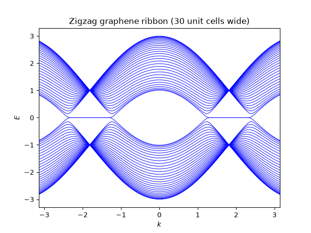
Kane-Mele ribbon: edge-state crossing near k=1.8188, E=0.00484.
Bulk gap at k=0 (far from the edge-state crossing): 1.0096.

(-3.141592653589793, 3.141592653589793)