Anderson Localization

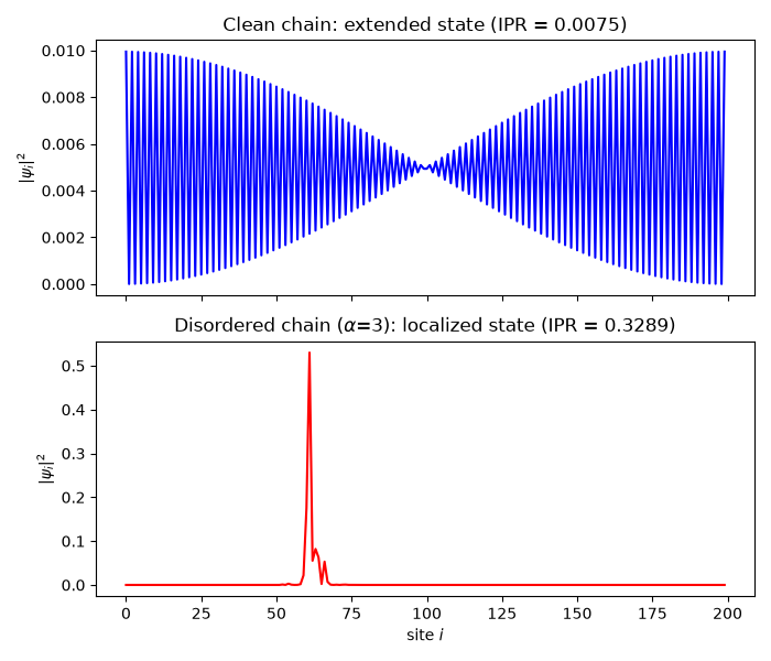
In a 1D (or 2D) tight-binding chain, any nonzero amount of uncorrelated onsite disorder exponentially localizes every eigenstate – interference between all the scattering paths off the random potential, rather than merely reducing a mean free path. A state’s degree of localization is diagnosed by its Inverse Participation Ratio,

\[\mathrm{IPR}_n = \frac{\sum_i |\psi_i^{(n)}|^4} {\left(\sum_i |\psi_i^{(n)}|^2\right)^2},\]

which is \(O(1/N)\) for a state extended over all N sites, and \(O(1)\) for a state localized on a handful of them – tbkit.system.System.get_ipr() computes it.

import numpy as np
import matplotlib.pyplot as plt

from tbkit.lattice import Lattice
from tbkit.system import System
from tbkit.plot import Plot


N = 200


def anderson_chain(alpha, seed, n=N):
    '''A 1D tight-binding chain with uniform onsite disorder of strength alpha.'''
    lat = Lattice(unit_cell=[{'tag': 'a', 'r0': (0., 0.)}], prim_vec=[(1., 0.)])
    lat.get_lattice(n1=n)
    sys = System(lat)
    sys.set_hopping([{'n': 1, 't': 1.}])
    sys.set_onsite({'a': 0.})
    if alpha > 0:
        rng_state = np.random.get_state()
        np.random.seed(seed)
        sys.set_onsite_dis(alpha=alpha)
        np.random.set_state(rng_state)
    sys.get_ham()
    sys.get_eig(eigenvec=True)
    sys.get_ipr()
    return sys

The chain

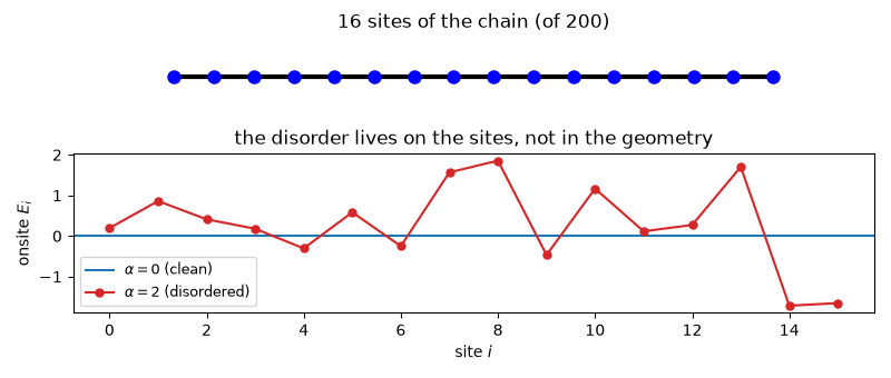
A plain 1D chain with uniform nearest-neighbor hopping. Only a short stretch is drawn: at the full 200 sites the markers overlap into an unreadable solid bar. The disorder is added to the onsite energies, so the geometry never changes – only what sits on each site, which is what the lower panel shows.

n_draw = 16
fig0, (ax_lat, ax_pot) = plt.subplots(2, 1, figsize=(8, 3.4),
                                                  gridspec_kw={'height_ratios': [1, 2]})
Plot(anderson_chain(alpha=0., seed=0, n=n_draw)).lattice(plt_hop=True, ms=9,
                                                                                  ax=ax_lat)
ax_lat.set_title('{} sites of the chain (of {})'.format(n_draw, N), fontsize=12)
ax_pot.axhline(0., color='C0', lw=1.5, label=r'$\alpha=0$ (clean)')
ax_pot.plot(np.arange(n_draw),
                 anderson_chain(alpha=2., seed=0, n=n_draw).onsite.real,
                 'o-', color='C3', ms=5, label=r'$\alpha=2$ (disordered)')
ax_pot.set_xlabel('site $i$')
ax_pot.set_ylabel('onsite $E_i$')
ax_pot.set_title('the disorder lives on the sites, not in the geometry',
                        fontsize=12)
ax_pot.legend(fontsize=9)
fig0.tight_layout()

Mean IPR grows sharply with disorder strength

Extended states become localized as the disorder strength grows.

alphas = np.linspace(0., 5., 21)
mean_ipr = np.array([anderson_chain(alpha, seed=0).ipr.mean() for alpha in alphas])

print('Clean chain (alpha=0): mean IPR = {:.5f} (expect ~ 1/N = {:.5f}, extended states).'
           .format(mean_ipr[0], 1/N))
print('Strongly disordered (alpha=5): mean IPR = {:.5f} (localized states).'.format(mean_ipr[-1]))
assert mean_ipr[0] < 3./N
assert mean_ipr[-1] > 50 * mean_ipr[0]
assert np.all(np.diff(mean_ipr) >= -1e-9)  # IPR grows (weakly) monotonically with disorder
print('IPR grows monotonically with disorder strength: OK')

fig, ax = plt.subplots()
ax.plot(alphas, mean_ipr, 'o-b')
ax.set_xlabel(r'disorder strength $\alpha$')
ax.set_ylabel('mean IPR')
ax.set_title('Anderson localization: IPR vs. disorder strength')

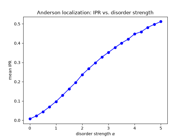
Clean chain (alpha=0): mean IPR = 0.00746 (expect ~ 1/N = 0.00500, extended states).
Strongly disordered (alpha=5): mean IPR = 0.51196 (localized states).
IPR grows monotonically with disorder strength: OK

Text(0.5, 1.0, 'Anderson localization: IPR vs. disorder strength')

Side by side: an extended state vs. a localized one

sys_clean = anderson_chain(alpha=0., seed=0)
sys_disordered = anderson_chain(alpha=3., seed=2)

# a mid-band state in each (band-center states localize first/most strongly).
i_clean = N // 2
i_dis = N // 2
intensity_clean = np.abs(sys_clean.rn[:, i_clean]) ** 2
intensity_dis = np.abs(sys_disordered.rn[:, i_dis]) ** 2

fig2, (ax1, ax2) = plt.subplots(2, 1, figsize=(7, 6), sharex=True)
ax1.plot(intensity_clean, 'b')
ax1.set_title('Clean chain: extended state (IPR = {:.4f})'.format(sys_clean.ipr[i_clean]))
ax1.set_ylabel(r'$|\psi_i|^2$')
ax2.plot(intensity_dis, 'r')
ax2.set_title(r'Disordered chain ($\alpha$=3): localized state (IPR = {:.4f})'
                        .format(sys_disordered.ipr[i_dis]))
ax2.set_xlabel('site $i$')
ax2.set_ylabel(r'$|\psi_i|^2$')
fig2.tight_layout()