The Haldane Model: Berry Curvature and a Topological Phase Transition

The Haldane model is honeycomb graphene with a complex next-nearest-neighbor hopping \(t_2 e^{i\phi}\) (breaking time-reversal symmetry, e.g. via a staggered flux pattern with zero net flux) and a staggered sublattice onsite energy \(\pm M\) (breaking inversion symmetry). It is the first model shown to realize a Chern insulator – a gapped phase with quantized Hall conductance and no net magnetic field.

The topological/trivial phase boundary sits at \(|M| = \sqrt{3}\,t_2\,|\sin\phi|\) (for this particular choice of which 3 next-nearest-neighbor vectors carry the phase \(+\phi\) vs. \(-\phi\) – the prefactor is convention-dependent and was pinned down numerically below, rather than assumed): the lower band’s Chern number, computed via chern_number(), is \(\pm 1\) for \(|M|\) below that, 0 above it.

import numpy as np
import matplotlib.pyplot as plt

from tbkit.lattice import Lattice
from tbkit.kspace import KSpace, reciprocal_vectors
from tbkit.system import System
from tbkit.plot import Plot


DX, DY = 0.5 * 3 ** 0.5, 0.5
unit_cell = [{'tag': 'a', 'r0': (0., 0.)}, {'tag': 'b', 'r0': (DX, DY)}]
prim_vec = [(2*DX, 0.), (DX, 1.5)]
t1, t2, phi = 1., 0.2, np.pi / 2
M_c = np.sqrt(3) * t2 * abs(np.sin(phi))  # critical mass (see module docstring)


def haldane(M):
    '''Build the Haldane model with staggered onsite energy +-M.'''
    lat = Lattice(unit_cell=unit_cell, prim_vec=prim_vec)
    hal = KSpace(lat)
    hal.set_hopping([{'i': 0, 'j': 1, 'R': (0, 0), 't': t1},
                            {'i': 0, 'j': 1, 'R': (-1, 0), 't': t1},
                            {'i': 0, 'j': 1, 'R': (0, -1), 't': t1}])
    # next-nearest-neighbor hopping: same 3 lattice vectors for both
    # sublattices, but with opposite chirality (t2*exp(+-i*phi)) -- this
    # circulating "staggered flux" is what breaks time-reversal symmetry
    # without any net magnetic field through the unit cell.
    for R in [(1, 0), (0, 1), (1, -1)]:
        hal.set_hopping([{'i': 0, 'j': 0, 'R': R, 't': t2*np.exp(1j*phi)}])
        hal.set_hopping([{'i': 1, 'j': 1, 'R': R, 't': t2*np.exp(-1j*phi)}])
    hal.set_onsite({'a': M, 'b': -M})
    return hal

The lattice

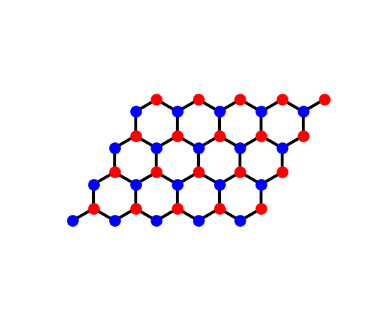
The Haldane model lives on the plain honeycomb lattice – two orbitals per unit cell, drawn in two colours below, with the nearest-neighbor bonds shown. What the model adds is invisible in this picture: a second-neighbor hopping within each sublattice, complex and of opposite chirality on the two, which is why it breaks time-reversal symmetry without any net flux through the cell.

patch = Lattice(unit_cell=unit_cell, prim_vec=prim_vec)
patch.get_lattice(n1=5, n2=4)
vis = System(patch)
vis.set_hopping([{'n': 1, 't': t1}])
fig_lat = Plot(vis).lattice(plt_hop=True, ms=12, figsize=(5.5, 4.5))

Chern number across the topological phase transition

masses = np.linspace(0., 2*M_c, 21)
chern = [haldane(M).chern_number(bands=[0], nk=40) for M in masses]

print('Critical mass M_c = sqrt(3)*t2*sin(phi) = {:.4f}'.format(M_c))
print('Chern number at M=0            (topological): {:.4f}'.format(chern[0]))
print('Chern number at M=2*M_c        (trivial):      {:.4f}'.format(chern[-1]))
assert np.isclose(chern[0], 1., atol=1e-2)
assert np.isclose(chern[-1], 0., atol=1e-2)
print('Phase transition reproduced: C = 1 (topological) -> C = 0 (trivial). OK')

fig, ax = plt.subplots()
ax.plot(masses/M_c, chern, 'o-b')
ax.axvline(1., color='k', ls='--', lw=1)
ax.set_xlabel('$M/M_c$')
ax.set_ylabel('Chern number (lower band)')
ax.set_title('Haldane model: topological phase transition')

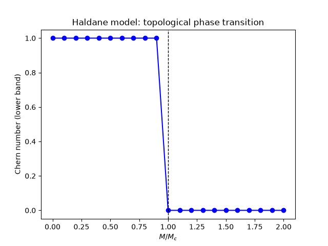
Critical mass M_c = sqrt(3)*t2*sin(phi) = 0.3464
Chern number at M=0            (topological): 1.0000
Chern number at M=2*M_c        (trivial):      0.0000
Phase transition reproduced: C = 1 (topological) -> C = 0 (trivial). OK

Text(0.5, 1.0, 'Haldane model: topological phase transition')

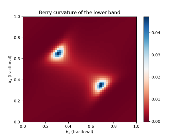
Berry curvature in the topological phase

berry_curvature() concentrates near the Dirac points (where the gap is smallest), with total flux \(2\pi\).

hal_topological = haldane(M=0.)
curv = hal_topological.berry_curvature(bands=[0], nk=60)
fig2, ax2 = plt.subplots()
im = ax2.imshow(curv.T, origin='lower', extent=[0, 1, 0, 1], aspect='auto', cmap='RdBu')
ax2.set_xlabel('$k_1$ (fractional)')
ax2.set_ylabel('$k_2$ (fractional)')
ax2.set_title('Berry curvature of the lower band')
fig2.colorbar(im, ax=ax2)

<matplotlib.colorbar.Colorbar object at 0x116056120>

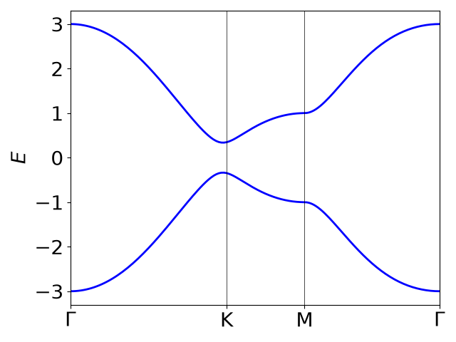
Band structure in the topological phase

b1, b2 = (np.array(v) for v in reciprocal_vectors(prim_vec))
Gamma, K, M_pt = np.zeros(2), (b1 - b2) / 3, b1 / 2
hal_topological.k_path([Gamma, K, M_pt, Gamma], nk=60)
fig3 = hal_topological.plot_bands(node_labels=[r'$\Gamma$', 'K', 'M', r'$\Gamma$'])