The Recursive Green’s Function: Localization Length of Long Disordered Wires

The Landauer transmission of a device needs its Green’s function between the two leads. Inverting the whole device matrix costs \(N^3\) for \(N\) sites, which rules out the long samples in which localization shows. In 1981 Thouless and Kirkpatrick, Lee and Fisher, and MacKinnon and Kramer cut the sample into slices coupled only to their neighbours and added them one at a time,

\[g_i = [E - H_{ii} - H_{i,i-1}\,g_{i-1}H_{i-1,i}]^{-1}\, ,\qquad G_{i1} = g_iH_{i,i-1}G_{i-1,1}\, ,\]

so that \(T = \mathrm{Tr}[\Gamma_RG_{N1}\Gamma_LG_{N1}^\dagger]\) costs a time linear in the length and only slice-sized inversions. With it, MacKinnon and Kramer followed the conductance of quasi-1D bars over thousands of slices and extracted the localization length that underlies one-parameter scaling.

RecursiveTransport implements it; it agrees with the dense Transport wherever both apply.

import numpy as np
import matplotlib.pyplot as plt
import scipy.sparse as sp

import tbkit.lattices as lattices
from tbkit.kspace import ribbon
from tbkit.plot import Plot
from tbkit.system import System
from tbkit.transport import Transport, RecursiveTransport, lead_from_kspace, slices_from_positions

t = -1.
rng = np.random.default_rng(1)

The same numbers as the dense inversion

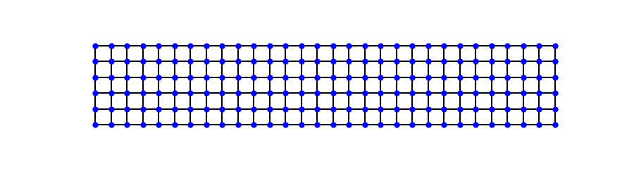
A disordered square-lattice strip, 30 x 6 sites, between two clean strips of the same width.

length, width = 30, 6
lat = lattices.square()
lat.get_lattice(length, width)
sys = System(lat)
sys.set_hopping([{'n': 1, 't': t}])
sys.set_onsite({'a': 0.})
sys.onsite[:] = 2. * (rng.random(lat.sites) - 0.5)
sys.get_ham()
# the strip, with its nearest-neighbour bonds (the random onsite energies
# are not drawn); each column of six sites is one slice of the recursion
fig_lat = Plot(sys).lattice(plt_hop=True, ms=6, c=1.5, figsize=(9, 2.4))

The recursive and the dense transmissions:

strip = ribbon(lattices.square(), [{'i': 0, 'j': 0, 'R': (1, 0), 't': t},
                                               {'i': 0, 'j': 0, 'R': (0, 1), 't': t}], width=width, direction=1)
(h_l, v_l), (h_r, v_r) = lead_from_kspace(strip, -1), lead_from_kspace(strip, 1)
slices = slices_from_positions(lat.coor['x'])  # columns; sites of a column by increasing y
dense = Transport(sys.ham)
dense.add_lead(h_l, v_l, t * np.eye(width), slices[0])
dense.add_lead(h_r, v_r, t * np.eye(width), slices[-1])
rgf = RecursiveTransport(sys.ham, slices, (h_l, v_l, t * np.eye(width)), (h_r, v_r, t * np.eye(width)))
energies = np.linspace(-3.8, 3.8, 39)
assert np.allclose(rgf.transmission(energies), dense.transmission(energies), atol=1e-9)
print('recursive and dense transmissions agree at every energy')

recursive and dense transmissions agree at every energy

Anderson localization in a chain, thousands of sites long

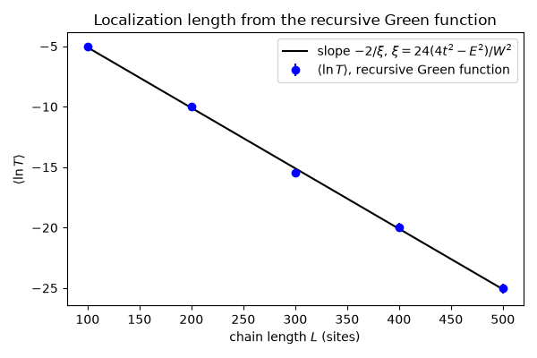
In one dimension every state is localized: the typical transmission decays as \(\langle\ln T\rangle = -2L/\xi\). For weak box disorder of width \(W\), perturbation theory (Thouless 1979) gives \(\xi(E) = 24(4t^2 - E^2)/W^2\) – 40 sites for \(W = 1.5\), \(E = 0.5\). Chains up to 12 localization lengths long, 300 disorder samples each:

W, energy = 1.5, 0.5
lengths = np.arange(100, 501, 100)
chain = lattices.chain()
chain.get_lattice(int(lengths.max()))
clean = System(chain)
clean.set_hopping([{'n': 1, 't': t}])
clean.set_onsite({'a': 0.})
clean.get_ham()
lead = ([[0.]], [[t]], [[t]])
log_t = np.zeros((len(lengths), 300))
for a, n in enumerate(lengths):
    ham = clean.ham[:n, :n]
    one_site = [[i] for i in range(n)]
    for b in range(log_t.shape[1]):
        wire = RecursiveTransport(ham + sp.diags(W * (rng.random(n) - 0.5)), one_site, lead, lead)
        log_t[a, b] = np.log(wire.transmission(energy)[0])
slope = np.polyfit(lengths, log_t.mean(axis=1), 1)[0]
xi = -2 / slope
xi_thouless = 24 * (4 * t ** 2 - energy ** 2) / W ** 2
print('localization length {:.1f} sites (Thouless: {:.1f})'.format(xi, xi_thouless))
assert abs(xi / xi_thouless - 1) < 0.1

localization length 40.0 sites (Thouless: 40.0)

A wire of 100 000 sites

A strip 20 sites wide and 5000 long would need a dense matrix of 160 GB; slice by slice it takes a fraction of a second. Over that length even weak disorder (\(W = 0.5\)) cuts the transmission far below the number of open channels.

length, width = 5000, 20
column = t * (np.eye(width, k=1) + np.eye(width, k=-1))
ham = (sp.kron(sp.eye(length), column) + sp.kron(sp.eye(length, k=1) + sp.eye(length, k=-1),
                                                                   t * sp.eye(width))
          + sp.diags(0.5 * (rng.random(length * width) - 0.5))).tocsr()
cols = [list(range(c * width, (c + 1) * width)) for c in range(length)]
strip = ribbon(lattices.square(), [{'i': 0, 'j': 0, 'R': (1, 0), 't': t},
                                               {'i': 0, 'j': 0, 'R': (0, 1), 't': t}], width=width, direction=1)
(h_l, v_l), (h_r, v_r) = lead_from_kspace(strip, -1), lead_from_kspace(strip, 1)
long_wire = RecursiveTransport(ham, cols, (h_l, v_l, t * np.eye(width)), (h_r, v_r, t * np.eye(width)))
e_wire = -1.
channels = sum(abs(e_wire - 2 * t * np.cos(m * np.pi / (width + 1))) < 2 * abs(t) for m in range(1, width + 1))
t_wire = long_wire.transmission(e_wire, eta=1e-12)[0]
print('{} sites: T = {:.2f} for {} open channels'.format(length * width, t_wire, channels))
assert 0.05 < t_wire < 0.5 * channels

fig, ax = plt.subplots(figsize=(6, 4))
ax.errorbar(lengths, log_t.mean(axis=1), yerr=log_t.std(axis=1) / np.sqrt(log_t.shape[1]), fmt='ob',
                label=r'$\langle\ln T\rangle$, recursive Green function')
ax.plot(lengths, -2 * lengths / xi_thouless + np.mean(log_t.mean(axis=1) + 2 * lengths / xi_thouless), '-k',
          label=r'slope $-2/\xi$, $\xi = 24(4t^2-E^2)/W^2$')
ax.set_xlabel('chain length $L$ (sites)')
ax.set_ylabel(r'$\langle\ln T\rangle$')
ax.set_title('Localization length from the recursive Green function')
ax.legend()
fig.set_layout_engine('tight')

100000 sites: T = 0.23 for 14 open channels