Projected Bands and Spin Textures

A band structure says where the states are in energy; their character says what they are made of. A “fat band” plot colors each band by its weight on a sublattice, an orbital or a spin direction,

\[w_n(\mathbf{k}) = \langle u_n(\mathbf{k})|P|u_n(\mathbf{k})\rangle,\]

computed by band_weights() and drawn by plot_bands() with weights=. For a spin-orbit coupled band, the spin expectation value along a constant-energy contour is its spin texture (spin_texture(), plot_spin_texture()). The k-paths come from high_symmetry_path(), which recognizes the Bravais lattice and returns the standard high-symmetry points with their labels.

import numpy as np

import tbkit.lattices as lattices
from tbkit.lattice import Lattice
from tbkit.bridges import finite_system
from tbkit.kspace import KSpace, PAULI, high_symmetry_path
from tbkit.plot import Plot
from tbkit.system import System

Gapped graphene: the valleys are sublattice polarized

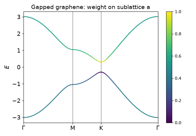
A staggered potential \(\pm m\) on the two sublattices (hexagonal boron nitride, or graphene on it) opens a gap \(2m\) at the Dirac points. At K and K’ the two sublattices decouple, so the lower band lives entirely on sublattice b (onsite \(-m\)) and the upper one on a. Away from the valleys the bands mix both, half and half at \(m = 0\).

DX = np.sqrt(3) / 2
lat = Lattice(unit_cell=[{'tag': 'a', 'r0': (0., 0.)}, {'tag': 'b', 'r0': (DX, 0.5)}],
                  prim_vec=[(2 * DX, 0.), (DX, 1.5)])
mass = 0.3
gra = KSpace(lat)
gra.set_hopping([{'i': 0, 'j': 1, 'R': R, 't': -1.} for R in [(0, 0), (-1, 0), (0, -1)]])
gra.set_onsite({'a': mass, 'b': -mass})

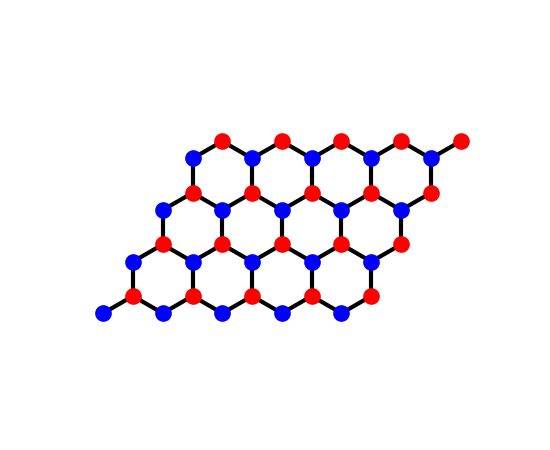
The model on a patch of \(5\times4\) cells (finite_system()): the honeycomb lattice with its nearest-neighbour bonds, sublattice a (onsite \(+m\)) and b (\(-m\)) in two colours.

fig_lat = Plot(finite_system(gra, (5, 4))).lattice(plt_hop=True, ms=12, figsize=(5.5, 4.5))

The bands, coloured by their weight on sublattice a:

points, labels = high_symmetry_path(lat)
print('Path:', labels)
nk = 60
gra.k_path(points, nk=nk)
weight_a = gra.band_weights('a')
k_index = 2 * nk  # K, the third point of Gamma - M - K - Gamma
print('Weight on sublattice a at K: lower band {:.2e}, upper band {:.6f}'.format(*weight_a[k_index]))
assert np.allclose(weight_a[k_index], [0., 1.], atol=1e-12)
assert np.allclose(gra.en[k_index], [-mass, mass])
# the weights on the two sublattices add up to one
assert np.allclose(weight_a + gra.band_weights('b'), 1.)

fig = gra.plot_bands(node_labels=labels, weights=weight_a, fs=14, figsize=(6.5, 4.5))
fig.axes[0].set_title('Gapped graphene: weight on sublattice a', fontsize=14)

Path: ['$\\Gamma$', 'M', 'K', '$\\Gamma$']
Weight on sublattice a at K: lower band 1.37e-30, upper band 1.000000

Text(0.5, 1.0, 'Gapped graphene: weight on sublattice a')

Rashba spin-orbit coupling: spin-momentum locking

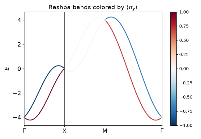
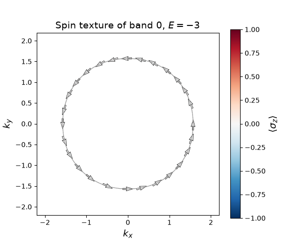
A square lattice without inversion symmetry (a surface, an interface) acquires the Rashba coupling \(H_R = 2\alpha(\sin k_y\,\sigma_x - \sin k_x\,\sigma_y)\): an effective magnetic field in the plane, perpendicular to the momentum, which splits every band in two. Each branch has its spin locked perpendicular to \((\sin k_x, \sin k_y)\) – along \(\pm\sigma_y\) on the \(\Gamma\)-X line, the lower branch along \(+\sigma_y\) – and the two branches wind in opposite directions around the Fermi contour.

alpha = 0.5
ras = KSpace(lattices.square(), spin=True)
ras.set_hopping([{'i': 0, 'j': 0, 'R': (1, 0), 't': -np.eye(2) + 1j * alpha * PAULI['y']},
                       {'i': 0, 'j': 0, 'R': (0, 1), 't': -np.eye(2) - 1j * alpha * PAULI['x']}])

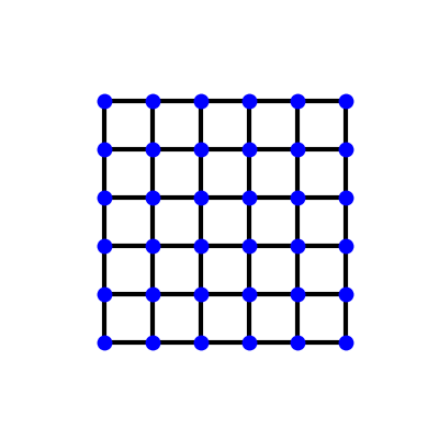
The square lattice, one spin-1/2 site per cell, with its nearest-neighbour bonds; each carries the hopping and the Rashba spin flip (not drawn).

patch = lattices.square()
patch.get_lattice(n1=6, n2=6)
vis = System(patch)
vis.set_hopping([{'n': 1, 't': -1.}])
fig_lat_sq = Plot(vis).lattice(plt_hop=True, ms=10, figsize=(4, 4))

The bands, coloured by \(\langle\sigma_y\rangle\):

points, labels = high_symmetry_path(ras.lat)
ras.k_path(points, nk=nk)
sigma_y = ras.band_weights(ras.spin_operator('y'))
gamma_x = slice(1, nk)  # inside Gamma - X (Gamma and X are Kramers degenerate)
assert np.allclose(sigma_y[gamma_x], [1., -1.])
fig2 = ras.plot_bands(node_labels=labels, weights=sigma_y, fs=14, figsize=(6.5, 4.5))
fig2.axes[0].set_title(r'Rashba bands colored by $\langle\sigma_y\rangle$', fontsize=14)

# the spin texture of the lower branch on its contour E = -3t
segs = ras.fermi_surface(-3., nk=100, bands=0)[0]
k_contour = segs.mean(axis=1)
spin = ras.spin_texture(k_contour, band=0)
assert np.allclose(np.linalg.norm(spin, axis=1), 1.) and np.allclose(spin[:, 2], 0.)
assert np.allclose(np.sum(spin[:, :2] * np.sin(k_contour), axis=1), 0., atol=1e-10)
# counterclockwise winding for the lower branch, clockwise for the upper one
def winding(s):
    return k_contour[:, 0] * s[:, 1] - k_contour[:, 1] * s[:, 0]  # (k x s)_z


assert np.all(winding(spin) > 0) and np.all(winding(ras.spin_texture(k_contour, 1)) < 0)
print('Lower branch: in-plane spin, perpendicular to (sin kx, sin ky), winding counterclockwise.')

fig3 = ras.plot_spin_texture(0, energy=-3., n_arrows=32, fs=14, figsize=(6, 5))

• 
• 

Lower branch: in-plane spin, perpendicular to (sin kx, sin ky), winding counterclockwise.