Thermoelectric Transport: the Mott Formula and the Wiedemann-Franz Law

Sivan and Imry (1986) extended the Landauer formula to heat: a temperature difference across a phase-coherent conductor drives a current, and a bias carries heat. In linear response, every coefficient is a moment of the transmission over the Fermi window,

\[L_n = \int dE\,(E - \mu)^n\,T(E)\left(-\frac{\partial f}{\partial E}\right)\, , \qquad G = L_0\, ,\quad S = -\frac{L_1}{TL_0}\, ,\quad \kappa = \frac{1}{T}\left(L_2 - \frac{L_1^2}{L_0}\right)\, .\]

When \(T(E)\) is smooth on the scale \(k_BT\), the Sommerfeld expansion gives the Mott formula \(S = -\frac{\pi^2}{3}k_BT\, \frac{d\ln T}{dE}\) and the Wiedemann-Franz law \(\kappa = \frac{\pi^2}{3} TG\). A transmission sharper than \(k_BT\) breaks both. A narrow resonance filters energies, carries charge with almost no heat, and drives the Lorenz ratio to zero (Mahan and Sofo 1996).

thermoelectric() computes \(G\), \(S\) and \(\kappa\) from the exact transmission (smatrix()). Here it is applied to a resonant level between two chains. Units: \(k_B = 1\), \(G\) in \(e^2/h\), \(S\) in \(k_B/e\).

import numpy as np
import matplotlib.pyplot as plt

from tbkit.lattice import Lattice
from tbkit.plot import Plot
from tbkit.system import System
from tbkit.transport import Transport


t_dot, e_dot = 0.1, 0.3
lorenz = np.pi**2 / 3
ham = np.array([[0., t_dot, 0.], [t_dot, e_dot, t_dot], [0., t_dot, 0.]])
dot = Transport(ham)
dot.add_lead([[0.]], [[1.]], [[1.]], [0])
dot.add_lead([[0.]], [[1.]], [[1.]], [2])

The lattice

A single level (red) between two semi-infinite chains (blue, four sites of each drawn), bond widths proportional to the hoppings: \(1\) along the chains, \(t_{dot} = 0.1\) to the level.

lat_vis = Lattice(unit_cell=[{'tag': 'a', 'r0': (0., 0.)}], prim_vec=[(1., 0.)])
lat_vis.get_lattice(n1=9)
lat_vis.remove_sites([4])
lat_vis.add_sites(np.array([(4., 0., 'b')], dtype=lat_vis.dtype))
vis = System(lat_vis)
vis.set_hopping([{'n': 1, 'tag': 'aa', 't': 1.}, {'n': 1, 'tag': 'ab', 't': t_dot},
                      {'n': 1, 'tag': 'ba', 't': t_dot}])
fig_lat = Plot(vis).lattice(plt_hop=True, ms=12, c=4., figsize=(7, 1.2))

A resonant level

The level \(\varepsilon_0\), weakly coupled to the chains, transmits fully at its resonance \(E_r\) (shifted by the leads), within a width \(\Gamma\).

energies = np.linspace(0.1, 0.5, 4001)
trans = dot.transmission(energies)
e_r = energies[np.argmax(trans)]
half = energies[trans > 0.5]
width = half[-1] - half[0]
assert trans.max() > 0.9999 and 0.03 < width < 0.06
print('Resonance at E_r = {:.4f}, width Gamma = {:.4f}.'.format(e_r, width))

Resonance at E_r = 0.3030, width Gamma = 0.0398.

Low temperature: Mott and Wiedemann-Franz

At \(k_BT = \Gamma/50\), \(G(\mu)\) follows \(T(\mu)\). The thermopower changes sign at the resonance, with electrons (\(S < 0\)) below it and holes above it, as the Mott formula predicts. The Lorenz ratio \(\kappa/(TG)\) is \(\pi^2/3\).

kt = width / 50
mus = e_r + width * np.linspace(-2., 2., 41)
coeffs = np.array([dot.thermoelectric(float(mu), kt) for mu in mus])
g, s, kappa = coeffs.T
h = 1e-5
mott = -lorenz * kt * (np.log(dot.transmission(mus + h)) - np.log(dot.transmission(mus - h))) / (2 * h)
assert np.allclose(g, dot.transmission(mus), rtol=0.02)
assert np.max(np.abs(s - mott)) < 0.02 * np.max(np.abs(mott))
assert np.all(s[mus < e_r - 0.1 * width] < 0) and np.all(s[mus > e_r + 0.1 * width] > 0)
assert np.allclose(kappa / (kt * g), lorenz, rtol=0.02)
print('k_B T = Gamma/50: Mott formula within 2%, Lorenz ratio = pi^2/3 within 2%.')

k_B T = Gamma/50: Mott formula within 2%, Lorenz ratio = pi^2/3 within 2%.

High temperature: an energy filter

Once \(k_BT \gg \Gamma\), the electrons that cross the level all have the energy \(E_r\). They carry charge but almost no heat at zero current, and the Lorenz ratio drops far below \(\pi^2/3\).

ratios = np.logspace(-2, 1, 13)
lorenz_ratio = []
for r in ratios:
    gg, _, kk = dot.thermoelectric(float(e_r), float(r * width))
    lorenz_ratio.append(kk / (r * width * gg) / lorenz)
lorenz_ratio = np.array(lorenz_ratio)
assert abs(lorenz_ratio[0] - 1) < 0.01 and lorenz_ratio[-1] < 0.01
assert np.all(np.diff(lorenz_ratio) < 1e-6)
print('Lorenz ratio / (pi^2/3): {:.4f} at k_B T = Gamma/100, {:.4f} at 10 Gamma.'.format(
    lorenz_ratio[0], lorenz_ratio[-1]))

fig, axes = plt.subplots(1, 3, figsize=(12, 3.6))
ax = axes[0]
ax.plot(energies, trans, 'k')
ax.axvspan(e_r - width / 2, e_r + width / 2, color='orange', alpha=0.3, label=r'$\Gamma$')
ax.set_xlim(e_r - 6 * width, e_r + 6 * width)
ax.set_xlabel('$E$')
ax.set_ylabel('$T(E)$')
ax.set_title('Resonant level')
ax.legend(fontsize=8)

ax = axes[1]
x = (mus - e_r) / width
ax.plot(x, g, 'k', label='$G$ ($e^2/h$)')
ax.plot(x, s, 'ob', ms=3, label='$S$ ($k_B/e$)')
ax.plot(x, mott, '-b', lw=0.8, label='Mott formula')
ax.axhline(0., color='gray', lw=0.5)
ax.set_xlabel(r'$(\mu - E_r)/\Gamma$')
ax.set_title(r'$k_BT = \Gamma/50$')
ax.legend(fontsize=8)

ax = axes[2]
ax.semilogx(ratios, lorenz_ratio, 'o-r', ms=4)
ax.axhline(1., color='gray', ls='--', lw=0.8)
ax.set_xlabel(r'$k_BT/\Gamma$')
ax.set_ylabel(r'$\kappa/(TG)\ /\ (\pi^2/3)$')
ax.set_title('Wiedemann-Franz law at $\\mu = E_r$')
fig.set_layout_engine('tight')

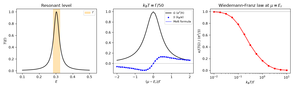
Lorenz ratio / (pi^2/3): 0.9959 at k_B T = Gamma/100, 0.0029 at 10 Gamma.