Fermi Surfaces and Constant-Energy Contours

The Fermi surface \(E_n(\mathbf{k}) = E_F\) separates the occupied states from the empty ones: transport, screening, magnetic oscillations and instabilities all happen on it. Its shape matters (nesting), and so does its topology: when the Fermi level crosses a saddle point of a band, the surface changes connectivity – a Lifshitz transition.

fermi_surface() computes the constant-energy lines (2D) or surfaces (3D) of the bands on a uniform mesh, by interpolating them linearly in triangles or tetrahedra and cutting each one exactly – the same decomposition as the tetrahedron density of states – and folds every piece into the first Brillouin zone. plot_fermi_surface() draws them, with the zone.

import numpy as np
import matplotlib.pyplot as plt
from matplotlib.collections import LineCollection
from mpl_toolkits.mplot3d.art3d import Line3DCollection

import tbkit.lattices as lattices
from tbkit.lattice import Lattice
from tbkit.bridges import finite_system
from tbkit.kspace import KSpace, high_symmetry_path
from tbkit.plot import Plot
from tbkit.system import System

The square lattice at half filling: a perfectly nested square

\(E = -2t(\cos k_x + \cos k_y) = 0\) is the square \(|k_x| + |k_y| = \pi\). The vector \(\mathbf{Q} = (\pi, \pi)\) maps each of its edges onto the opposite one (nesting), which drives the antiferromagnetic and charge-density-wave instabilities of the half-filled square lattice.

sq = KSpace(lattices.square())
sq.set_hopping([{'i': 0, 'j': 0, 'R': (1, 0), 't': -1.}, {'i': 0, 'j': 0, 'R': (0, 1), 't': -1.}])

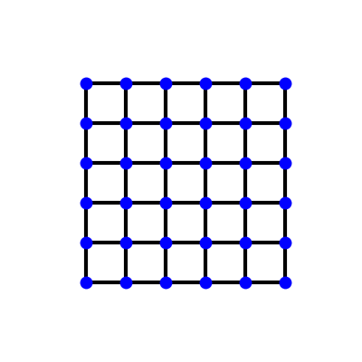
The square lattice, one site per cell with nearest-neighbour hopping, on \(6\times6\) cells (finite_system()):

fig_lat = Plot(finite_system(sq, (6, 6))).lattice(plt_hop=True, ms=10, figsize=(4, 4))

Its Fermi surface at half filling:

segs = sq.fermi_surface(0., nk=64)[0]
pts = segs.reshape(-1, 2)
assert np.allclose(np.abs(pts).sum(axis=1), np.pi)
# nesting: k + Q, brought back into the zone, lies on the surface again
shifted = (pts + np.pi + np.pi) % (2 * np.pi) - np.pi
assert np.allclose(np.abs(shifted).sum(axis=1), np.pi)
print('Half filling: |kx| + |ky| = pi on all {} segments, nested by Q = (pi, pi).'.format(len(segs)))

fig = sq.plot_fermi_surface(0., figsize=(5, 5), fs=14)

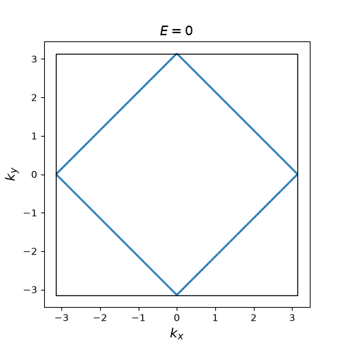
Half filling: |kx| + |ky| = pi on all 410 segments, nested by Q = (pi, pi).

Graphene: Dirac pockets, trigonal warping, a Lifshitz transition

Near the Dirac points the upper band is a cone \(E = v_F|\mathbf{q}|\), \(v_F = 3ta/2\) (\(a\) the carbon-carbon distance): the Fermi surface of slightly doped graphene is a circle of radius \(E/v_F\) around each zone corner. Further up the cones warp into triangles, and at \(E = t\) – the van Hove saddle point at M – the six pockets merge into one contour around \(\Gamma\).

DX = np.sqrt(3) / 2
lat = Lattice(unit_cell=[{'tag': 'a', 'r0': (0., 0.)}, {'tag': 'b', 'r0': (DX, 0.5)}],
                  prim_vec=[(2 * DX, 0.), (DX, 1.5)])
gra = KSpace(lat)
gra.set_hopping([{'i': 0, 'j': 1, 'R': R, 't': -1.} for R in [(0, 0), (-1, 0), (0, -1)]])

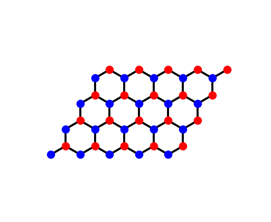
The honeycomb lattice, two sites per cell (sublattices ‘a’ and ‘b’, in two colours) and nearest-neighbour hopping, on \(5\times4\) cells (finite_system()):

fig_lat = Plot(finite_system(gra, (5, 4))).lattice(plt_hop=True, ms=12, figsize=(5.5, 4.5))

Its Fermi surfaces, below and above the Lifshitz transition:

points, labels = high_symmetry_path(lat)
M, K = points[1], points[2]
corners = [np.array([[np.cos(a), -np.sin(a)], [np.sin(a), np.cos(a)]]) @ K for a in np.arange(6) * np.pi / 3]


def distance_to_corners(e):
    p = gra.fermi_surface(e, nk=150, bands=1)[0].reshape(-1, 2)
    return np.min([np.linalg.norm(p - c, axis=1) for c in corners], axis=0)


for e in (0.2, 0.4):
    radius = distance_to_corners(e)
    print('E = {}: pocket radius {:.4f}, E/v_F = {:.4f}'.format(e, radius.mean(), e / 1.5))
    assert np.isclose(radius.mean(), e / 1.5, rtol=0.02)
warped = distance_to_corners(0.9)
print('E = 0.9: radius from {:.3f} to {:.3f} (trigonal warping)'.format(warped.min(), warped.max()))
assert warped.max() / warped.min() > 1.1
# the saddle point: E(M) = t
assert np.isclose(gra.get_bands([M])[0, 1], 1.)

fig2 = gra.plot_fermi_surface(0.3, bands=1, figsize=(5.5, 5), fs=14)
ax = fig2.axes[0]
ax.collections[0].set_label('$E = 0.3t$')
for e, color in ((0.9, 'C2'), (1.1, 'C3')):
    ax.add_collection(LineCollection(gra.fermi_surface(e, bands=1)[0], colors=color, lw=2,
                                                     label='$E = {}t$'.format(e)))
ax.legend(loc='center', fontsize=10)
ax.set_title('Graphene: Fermi surface vs doping', fontsize=14)

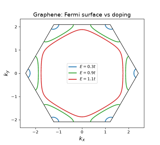
E = 0.2: pocket radius 0.1335, E/v_F = 0.1333
E = 0.4: pocket radius 0.2714, E/v_F = 0.2667
E = 0.9: radius from 0.547 to 0.842 (trigonal warping)

Text(0.5, 1.0, 'Graphene: Fermi surface vs doping')

The simple cubic lattice: from a sphere to an open surface

Near the bottom of \(E = -2t(\cos k_x + \cos k_y + \cos k_z)\) the Fermi surface is a small sphere around \(\Gamma\). At \(E = -2t\) it touches the zone faces at the X points (saddle points), and above, it is an open surface that runs through the faces into the next zone.

cubic = KSpace(Lattice(unit_cell=[{'tag': 'a', 'r0': (0., 0., 0.)}],
                              prim_vec=[(1., 0., 0.), (0., 1., 0.), (0., 0., 1.)]))
cubic.set_hopping([{'i': 0, 'j': 0, 'R': R, 't': -1.} for R in [(1, 0, 0), (0, 1, 0), (0, 0, 1)]])

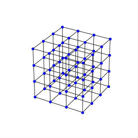
The simple cubic lattice, one site per cell and six nearest neighbours, here \(4\times4\times4\) sites of it:

lat_vis = Lattice(unit_cell=cubic.lat.unit_cell, prim_vec=cubic.lat.prim_vec)
lat_vis.get_lattice(4, 4, 4)
vis = System(lat_vis)
vis.set_hopping([{'n': 1, 't': 1.}])
pos = np.column_stack([lat_vis.coor[f] for f in 'xyz'])
bonds = np.stack([pos[vis.hop['i'].astype(int)], pos[vis.hop['j'].astype(int)]], axis=1)
fig_lat = plt.figure(figsize=(4.5, 4.5))
ax_lat = fig_lat.add_subplot(projection='3d')
ax_lat.add_collection3d(Line3DCollection(bonds, colors='k', linewidths=1))
ax_lat.scatter(*pos.T, s=30, c='b', depthshade=False)
ax_lat.set_aspect('equal')
ax_lat.set_axis_off()

A closed and an open Fermi surface:

closed = cubic.fermi_surface(-4., nk=30)[0]
opened = cubic.fermi_surface(-1., nk=30)[0]
print('E = -4: max |k_i| = {:.3f}; E = -1: max |k_i| = {:.3f} (pi = zone face)'.format(
    np.abs(closed).max(), np.abs(opened).max()))
assert np.abs(closed).max() < 0.9 * np.pi and np.isclose(np.abs(opened).max(), np.pi)

fig3 = cubic.plot_fermi_surface(-1., nk=30, figsize=(5.5, 5.5), fs=14)

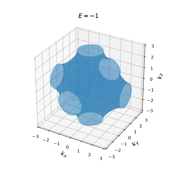
E = -4: max |k_i| = 1.571; E = -1: max |k_i| = 3.142 (pi = zone face)