Aharonov-Bohm Ring: A Magnetic Field on a Lattice

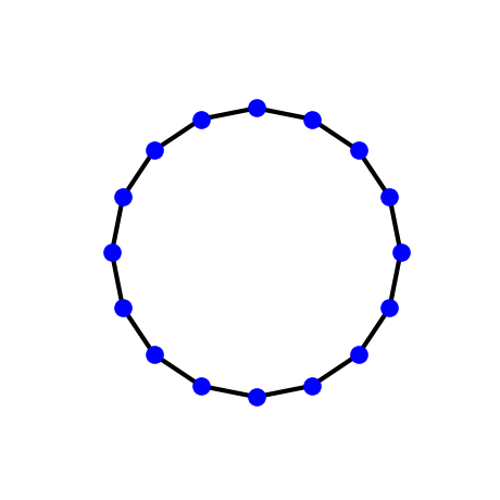
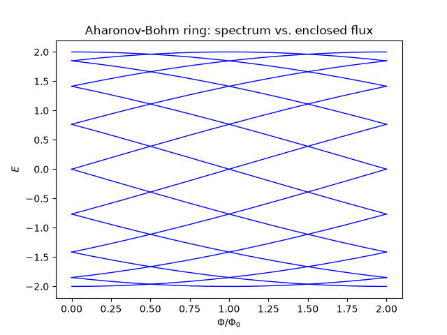
tbkit applies a magnetic field via the Peierls substitution (set_peierls_phase() / set_magnetic_field()): each hopping amplitude gets multiplied by a phase equal to the line integral of the vector potential along the bond. This script builds a simple N-site ring threaded by a perpendicular field and reproduces the textbook Aharonov-Bohm result: the energy spectrum is periodic in the flux threading the ring, with period exactly one flux quantum.

import numpy as np
import matplotlib.pyplot as plt

from tbkit.lattice import Lattice, COOR_DTYPE
from tbkit.system import System
from tbkit.plot import Plot

Building an N-site ring

A ring isn’t a Bravais lattice, so the sites are placed by hand and the hoppings wired up with set_hopping_manual().

N, R, t = 16, 3., 1.
theta = 2 * np.pi * np.arange(N) / N
coor = np.zeros(N, dtype=COOR_DTYPE)
coor['x'] = R * np.cos(theta)
coor['y'] = R * np.sin(theta)
coor['tag'] = 'a'

lat = Lattice(unit_cell=[{'tag': 'a', 'r0': (0., 0.)}], prim_vec=[(1., 0.)])
lat.add_sites(coor)

# add_sites() re-sorts lat.coor by (y, x), so site index i is no longer the
# i-th point placed above. Recover the ring order from the actual
# (now-shuffled) coordinates so the hoppings below connect true geometric
# neighbors around the ring.
angle = np.arctan2(lat.coor['y'], lat.coor['x']) % (2 * np.pi)
ring_order = np.argsort(angle)

sys = System(lat)
hop_dict = {(int(ring_order[k]), int(ring_order[(k + 1) % N])): t for k in range(N)}

sys.set_hopping_manual(hop_dict)

# The ring itself. The flux that matters below is the one enclosed by this
# polygon, not by the circle of radius R the sites were placed on.
fig_ring = Plot(sys).lattice(plt_hop=True, ms=12, figsize=(4.6, 4.6))

Sanity check at zero field: a ring of N sites has the analytic spectrum E_n = 2t cos(2 pi n / N).

sys.get_ham()
sys.get_eig()
expected = np.sort(2 * t * np.cos(2 * np.pi * np.arange(N) / N))
assert np.allclose(np.sort(sys.en.real), expected, atol=1e-8)
print('Zero-field spectrum matches E_n = 2t cos(2 pi n / N): OK')

Zero-field spectrum matches E_n = 2t cos(2 pi n / N): OK

Sweeping the flux through the ring

The Peierls phase accumulated around the ring encloses the polygon spanned by the N sites, not the continuous circle of radius R (the two only agree as N -> infinity). The exact area comes from the shoelace formula, so that “one flux quantum” means exactly one period below.

area = 0.5 * abs(np.sum(coor['x'] * np.roll(coor['y'], -1)
                                - np.roll(coor['x'], -1) * coor['y']))
n_flux = 201
fluxes = np.linspace(0., 2., n_flux)  # in units of the flux quantum
energies = np.zeros((n_flux, N))

for i, flux in enumerate(fluxes):
    sys.clear_hopping()
    sys.set_hopping_manual(hop_dict)
    sys.set_magnetic_field(alpha=flux / area)  # alpha = B/Phi_0 = flux / area
    sys.get_ham()
    sys.get_eig()
    energies[i] = sys.en.real

# The spectrum must be periodic in the flux with period 1 (one flux quantum).
half = n_flux // 2
assert np.allclose(np.sort(energies[0]), np.sort(energies[half]), atol=1e-6)
print('Spectrum is periodic in flux with period 1 flux quantum: OK')

fig, ax = plt.subplots()
for n in range(N):
    ax.plot(fluxes, energies[:, n], 'b', lw=1)
ax.set_xlabel(r'$\Phi/\Phi_0$')
ax.set_ylabel('$E$')
ax.set_title('Aharonov-Bohm ring: spectrum vs. enclosed flux')

Spectrum is periodic in flux with period 1 flux quantum: OK

Text(0.5, 1.0, 'Aharonov-Bohm ring: spectrum vs. enclosed flux')