

Note
Go to the end to download the full example code.
Flat-Band Ferromagnetism: Nagaoka, Mielke and Tasaki#
Itinerant ferromagnetism is hard to get from the Hubbard model: the repulsion \(U\) favours aligned spins, which cannot share a site, but aligning them costs kinetic energy. Three exact results say when the spins align fully anyway.
Nagaoka (1966). At \(U = \infty\), with one electron fewer than sites, the ground state is the saturated ferromagnet: the hole moves most freely through aligned spins. On a finite cluster this holds above a finite \(U_c\).
Mielke (1991). On line graphs such as the kagome lattice, the lowest band is exactly flat. Filled with electrons of one spin, it costs no kinetic energy over any other filling and no interaction energy at all (no site is doubly occupied): the saturated ferromagnet is a ground state for every \(U > 0\).
Tasaki (1992, 1995). Flat bands of other, decorated lattices do the same; and the ferromagnet survives when the flat band is bent into a nearly flat one, of width \(W\), provided \(U\) is large enough: the threshold grows with \(W\).
The first is checked by exact diagonalization of tiny clusters (a few
lines of second quantization below), the other two with
hubbard_mean_field() on a kagome()
torus.
import itertools

import numpy as np
import matplotlib.pyplot as plt
import scipy.sparse as sparse
import scipy.sparse.linalg as sla

import tbkit.lattices as lattices
from tbkit.meanfield import hubbard_mean_field
from tbkit.plot import Plot
from tbkit.system import System
Nagaoka: one hole in a square cluster#
With \(N_e = N - 1\) electrons, the Hubbard Hamiltonian is diagonalized in the sector \(S_z = 1/2\) (spin-up and spin-down Fock spaces of spinless fermions, coupled by \(U\)). Its lowest energy equals that of the fully polarized state – the \(N_e\) lowest single-particle levels, filled with one spin, which feel no \(U\) – exactly when the ground state has the maximal spin \(S = N_e/2\).
def fock_hopping(h, n_el):
    '''Hopping of n_el spinless fermions, and the occupations of the basis.'''
    basis = list(itertools.combinations(range(len(h)), n_el))
    index = {b: k for k, b in enumerate(basis)}
    occ = np.zeros((len(basis), len(h)))
    rows, cols, vals = [], [], []
    for k, b in enumerate(basis):
        occ[k, list(b)] = 1
        for j in b:
            for i in np.flatnonzero(h[:, j]):
                if i not in b:
                    lo, hi = sorted((i, j))
                    sign = (-1) ** sum(lo < m < hi for m in b)
                    rows.append(index[tuple(sorted(set(b) - {j} | {i}))])
                    cols.append(k)
                    vals.append(sign * h[i, j])
    return sparse.csr_matrix((vals, (rows, cols)), shape=(len(basis),) * 2), occ


def hubbard_ground_energy(h, U, n_el):
    '''Lowest energy of the Hubbard model at S_z = 1/2 (or 0).'''
    h_up, occ_up = fock_hopping(h, (n_el + 1) // 2)
    h_dn, occ_dn = fock_hopping(h, n_el // 2)
    ham = sparse.kron(h_up, sparse.identity(h_dn.shape[0])) \
        + sparse.kron(sparse.identity(h_up.shape[0]), h_dn) + U * sparse.diags((occ_up @ occ_dn.T).ravel())
    return sla.eigsh(ham, k=1, which='SA')[0][0]


def square_cluster(n1, n2):
    lat = lattices.square()
    lat.get_lattice(n1=n1, n2=n2)
    sys = System(lat)
    sys.set_hopping([{'n': 1, 't': -1.}])
    sys.get_ham()
    return sys.ham.toarray().real
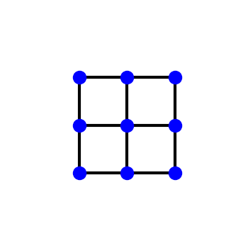
The largest cluster, a \(3\times3\) square of nine sites with nearest-neighbour hopping and open boundaries:
One hole in each cluster:
nagaoka = {}
for n1, n2 in ((2, 2), (3, 2), (3, 3)):
    h = square_cluster(n1, n2)
    n_el = len(h) - 1
    e_ferro = np.linalg.eigvalsh(h)[:n_el].sum()
    gaps = [hubbard_ground_energy(h, U, n_el) - e_ferro for U in (5., 1000.)]
    assert gaps[0] < -1e-3 and abs(gaps[1]) < 1e-8  # low spin at U = 5, S = N_e/2 at U = 1000
    if len(h) < 9:  # bisection for the threshold U_c
        lo, hi = 5., 1000.
        for _ in range(30):
            mid = np.sqrt(lo * hi)
            lo, hi = (mid, hi) if hubbard_ground_energy(h, mid, n_el) < e_ferro - 1e-9 else (lo, mid)
        nagaoka[len(h)] = hi
print('Nagaoka threshold: U_c = {:.2f}|t| (2x2), {:.1f}|t| (3x2); 3x3 saturated at U = 1000|t|.'
          .format(nagaoka[4], nagaoka[6]))
assert abs(nagaoka[4] - 18.58) < 0.01  # the known 4-site value
Nagaoka threshold: U_c = 18.58|t| (2x2), 51.8|t| (3x2); 3x3 saturated at U = 1000|t|.
Mielke: the flat band of the kagome lattice#
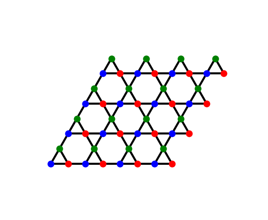
On a \(4\times4\) kagome torus (48 sites) with hopping \(t > 0\), the flat band at \(E = -2t\) holds 17 states (16, plus the one where it touches the next band). Seventeen electrons of one spin fill it.
The kagome lattice: three sites per unit cell (‘a’, ‘b’ and ‘c’, one per colour) on corner-sharing triangles. The bonds that close the torus are not drawn.
fig_kag = Plot(kagome_torus()).lattice(plt_hop=True, ms=10, figsize=(5.5, 4.5))
Mean field from a saturated and from a paramagnetic start:
def polarized_and_paramagnetic(sys, U, n_el):
    '''Mean-field solutions from a saturated and from a paramagnetic start.'''
    n = sys.lat.sites
    _, vec = np.linalg.eigh(sys.ham.toarray())
    up = np.sum(np.abs(vec[:, :n_el]) ** 2, axis=1)
    ferro = hubbard_mean_field(sys.ham, U, n_el, n_up=up, n_dn=np.zeros(n))
    para = hubbard_mean_field(sys.ham, U, n_el, n_up=np.full(n, n_el / (2 * n)), n_dn=np.full(n, n_el / (2 * n)))
    return ferro, para


sys = kagome_torus()
energies = np.linalg.eigvalsh(sys.ham.toarray())
n_flat = int(np.sum(np.isclose(energies, -2.)))
assert n_flat == 17 and np.all(energies[n_flat:] > -2. + 1e-6)
for U in (0.01, 0.5, 2., 8.):
    ferro, para = polarized_and_paramagnetic(sys, U, n_flat)
    # saturated, with the noninteracting energy -2t per electron: a ground state
    assert np.isclose(ferro.total_spin, n_flat / 2) and np.isclose(ferro.energy, -2. * n_flat)
    assert para.energy > ferro.energy and np.isclose(para.total_spin, 0.)
    # random starts reach other, higher, self-consistent solutions
    for seed in range(2):
        assert hubbard_mean_field(sys.ham, U, n_flat, seed=seed).energy > ferro.energy - 1e-9
print('Kagome flat band, 17 electrons: S = 17/2 and E = -34t for every U tried, down to 0.01t.')
Kagome flat band, 17 electrons: S = 17/2 and E = -34t for every U tried, down to 0.01t.
Tasaki: a nearly flat band needs a large enough U#
A second-neighbour hopping \(t_2\) bends the flat band, to a width \(W\). The saturated ferromagnet is then a mean-field solution, and beats the paramagnet, only above a threshold \(U_c\), here proportional to the width.
def saturated_wins(sys, U, n_el):
    ferro, para = polarized_and_paramagnetic(sys, U, n_el)
    return np.isclose(ferro.total_spin, n_el / 2) and ferro.energy < para.energy


widths, thresholds = [], []
for t2 in (0., -0.02, -0.05, -0.1, -0.15):
    sys = kagome_torus(t2)
    energies = np.linalg.eigvalsh(sys.ham.toarray())
    widths.append(energies[n_flat - 1] - energies[0])
    lo, hi = 0., 10.
    assert saturated_wins(sys, hi, n_flat)
    for _ in range(25):
        mid = (lo + hi) / 2
        lo, hi = (lo, mid) if saturated_wins(sys, mid, n_flat) else (mid, hi)
    thresholds.append(hi)
widths, thresholds = np.array(widths), np.array(thresholds)
for w, u in zip(widths, thresholds):
    print('W = {:.3f}t: U_c = {:.3f}t'.format(w, u))
ratio = thresholds[1:] / widths[1:]
print('U_c / W = {:.2f}, constant to {:.1%}.'.format(ratio.mean(), np.ptp(ratio) / ratio.mean()))
assert thresholds[0] < 1e-6 and np.allclose(ratio, ratio.mean(), rtol=0.01)

fig, axes = plt.subplots(1, 2, figsize=(10, 4))
axes[0].plot([4, 6], [nagaoka[4], nagaoka[6]], 'o-r')
axes[0].set_xlabel('sites N (one hole: N - 1 electrons)')
axes[0].set_ylabel(r'$U_c/|t|$')
axes[0].set_xticks([4, 6])
axes[0].set_title('Nagaoka: saturated ferromagnet above $U_c$')
axes[1].plot(widths, thresholds, 'o-b')
axes[1].set_xlabel(r'width $W$ of the lowest 17 states ($t$)')
axes[1].set_ylabel(r'$U_c/t$')
axes[1].set_title(r'Mielke ($W = 0$) and Tasaki: kagome, $4\times4$ torus')
fig.set_layout_engine('tight')
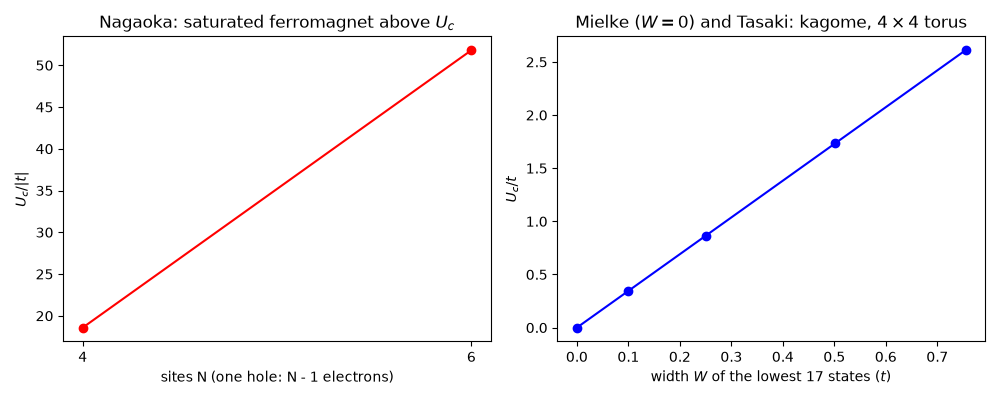
W = 0.000t: U_c = 0.000t
W = 0.100t: U_c = 0.346t
W = 0.251t: U_c = 0.866t
W = 0.502t: U_c = 1.736t
W = 0.755t: U_c = 2.610t
U_c / W = 3.46, constant to 0.1%.
Total running time of the script: (0 minutes 2.012 seconds)