Exceptional Points in Momentum Space: Complex Bands and the Bulk Fermi Arc

In a Hermitian 2D crystal, two bands touch at isolated diabolical points, such as graphene’s Dirac points. Add a non-Hermitian term (gain, loss, radiation into the environment) and each Dirac point is replaced by a pair of exceptional points (EPs), where the two eigenvalues and their eigenvectors coalesce. The complex bands \(E_\pm(\mathbf{k})\) are then the two sheets of a square root, \(E_\pm = \pm\sqrt{\Delta/4}\), and the EPs are its branch points. Each carries a topological charge: the winding of the discriminant \(\Delta(\mathbf{k}) = (E_+ - E_-)^2\) around it, \(\pm1\), or equivalently the eigenvalue vorticity \(\mp1/2\).

The two EPs are joined by a bulk Fermi arc: an open line on which the real parts of the two bands are equal, \(\mathrm{Re}(E_+ - E_-) = 0\), while their imaginary parts (lifetimes) differ – the non-Hermitian counterpart of a Fermi surface, which ends at the EPs instead of closing (Kozii and Fu 2017; observed in a photonic crystal by Zhou et al., Science 359, 1009 (2018)).

The model here is graphene with a non-Hermitian coupling \(i\gamma\,\sigma_x\) between the two sublattices of a cell,

\[H(\mathbf{k}) = \left[\mathrm{Re}f(\mathbf{k}) + i\gamma\right]\sigma_x - \mathrm{Im}f(\mathbf{k})\,\sigma_y\, ,\qquad E^2 = |f|^2 - \gamma^2 + 2i\gamma\,\mathrm{Re}f\, ,\]

with \(f(\mathbf{k}) = \sum_{\boldsymbol\delta}e^{i\mathbf{k}\cdot\mathbf{R}}\) the nearest-neighbour structure factor. The EPs are where \(E^2 = 0\): \(\mathrm{Re}f = 0\) and \(|\mathrm{Im}f| = \gamma\), and the Fermi arc is where \(E^2\) is real and negative: \(\mathrm{Re}f = 0\), \(|\mathrm{Im}f| < \gamma\). tbkit.exceptional.find_exceptional_points() and tbkit.exceptional.fermi_arcs() recover both numerically.

import numpy as np
import matplotlib.pyplot as plt

import tbkit.lattices as lattices
from tbkit.bridges import finite_system
from tbkit.kspace import KSpace
from tbkit.plot import Plot
import tbkit.exceptional as ex

gamma = 0.3
graphene = KSpace(lattices.honeycomb())
graphene.set_hopping([{'i': 0, 'j': 1, 'R': (0, 0), 't': 1.}, {'i': 0, 'j': 1, 'R': (-1, 0), 't': 1.},
                      {'i': 0, 'j': 1, 'R': (0, -1), 't': 1.}])
model = KSpace(lattices.honeycomb())
model.set_hopping([{'i': 0, 'j': 1, 'R': (0, 0), 't': 1.}, {'i': 0, 'j': 1, 'R': (-1, 0), 't': 1.},
                   {'i': 0, 'j': 1, 'R': (0, -1), 't': 1.}])
# i*gamma on both H_ab and H_ba: symmetric, not Hermitian
model.set_hopping([{'i': 0, 'j': 1, 'R': (0, 0), 't': 1j * gamma},
                   {'i': 1, 'j': 0, 'R': (0, 0), 't': 1j * gamma}], hermitian=False)
b1, b2 = (np.array(b) for b in model.rec_vec_k)
K = (b1 - b2) / 3


def f(k):
    '''Structure factor, H_ba of plain graphene.'''
    return graphene.get_ham(k)[1, 0]

The lattice

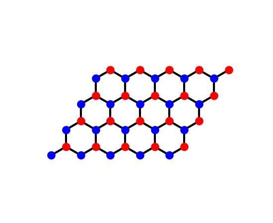
Graphene’s honeycomb lattice on a patch of \(5\times4\) cells (finite_system()): sublattices ‘a’ and ‘b’ in two colours, each bonded to its three nearest neighbours. The non-Hermitian term, \(i\gamma\) added to both directions of the intra-cell bond, adds no bond and is not drawn.

fig_lat = Plot(finite_system(graphene, (5, 4))).lattice(plt_hop=True, ms=12, figsize=(5.5, 4.5))

The exceptional points and their charges

The finder computes \(\Delta\) on a mesh of the Brillouin zone, locates the plaquettes around which it winds, and refines each zero by Newton’s method. Graphene’s two Dirac points, K and K’, each give a pair of EPs of opposite charge, so the charges add up to zero – the doubling theorem for EPs. Each point is second order (two eigenvalues coalesce, with a divergent Petermann factor) and sits exactly where \(\mathrm{Re}f = 0\) and \(|\mathrm{Im}f| = \gamma\).

eps = ex.find_exceptional_points(model, nk=40)
for k, q, order, kp in zip(eps.k, eps.charge, eps.order, eps.petermann):
    print('EP at k = ({:+.6f}, {:+.6f}): charge {:+d}, order {}, Petermann {:.1e}, '
          'Re f = {:.1e}, |Im f| = {:.10f}'.format(*k, q, order, kp, f(k).real, abs(f(k).imag)))
    assert abs(f(k).real) < 1e-8 and abs(abs(f(k).imag) - gamma) < 1e-8
assert len(eps.k) == 4 and sorted(eps.charge) == [-1, -1, 1, 1]
assert np.all(eps.order == 2) and np.all(eps.petermann > 1e8)
assert eps.total_charge == 0
# charge = discriminant winding = -2 x vorticity, on a small circle
for k, q in zip(eps.k, eps.charge):
    nu = ex.vorticity(model, ex.circle(k, 0.02))
    assert np.isclose(nu, -q / 2, atol=1e-10)
print('Total charge over the zone: {} (EPs come in pairs).'.format(eps.total_charge))

EP at k = (+1.055715, +1.971630): charge -1, order 2, Petermann 1.2e+15, Re f = 1.1e-16, |Im f| = 0.3000000000
EP at k = (+1.392260, +2.165934): charge +1, order 2, Petermann 4.6e+14, Re f = -2.8e-16, |Im f| = 0.3000000000
EP at k = (+2.235339, -0.071539): charge +1, order 2, Petermann 1.9e+15, Re f = 5.6e-17, |Im f| = 0.3000000000
EP at k = (+2.571884, +0.122766): charge -1, order 2, Petermann 3.4e+14, Re f = 2.2e-16, |Im f| = 0.3000000000
Total charge over the zone: 0 (EPs come in pairs).

The bulk Fermi arc

Along every edge of a mesh, the two eigenvalues are followed by continuation, and the points where their real parts cross are located by bisection. All of them lie on \(\mathrm{Re}f = 0\) between the two EPs, where \(|\mathrm{Im}f| < \gamma\) and the two bands have equal energy but different lifetimes, \(E_\pm = \pm i\sqrt{\gamma^2 - |f|^2}\).

arcs = ex.fermi_arcs(model, nk=60)
re_f = np.array([f(k).real for k in arcs])
im_f = np.array([abs(f(k).imag) for k in arcs])
en_arc = np.array([np.linalg.eigvals(model.get_ham(k)) for k in arcs])
print('{} points on the Fermi arcs: max |Re f| = {:.1e}, max |Im f| = {:.4f} < gamma'
      .format(len(arcs), np.abs(re_f).max(), im_f.max()))
assert len(arcs) > 10
assert np.abs(re_f).max() < 1e-8 and im_f.max() < gamma
assert np.allclose(en_arc.real, 0., atol=1e-8)
assert np.all(np.abs(en_arc[:, 0].imag - en_arc[:, 1].imag) > 1e-6)

22 points on the Fermi arcs: max |Re f| = 8.9e-16, max |Im f| = 0.2711 < gamma

Re E and Im E around a Dirac point

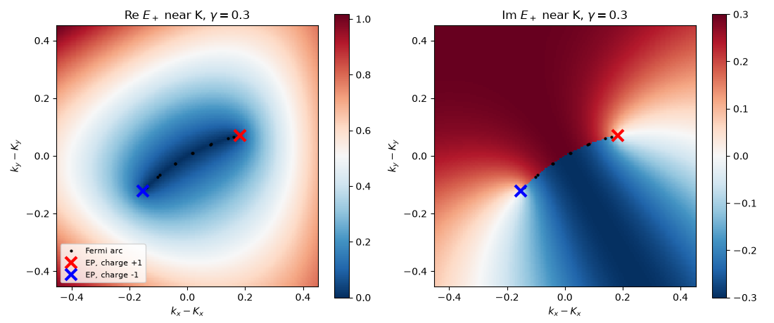
Near K, the upper sheet \(E_+\) (the eigenvalue with the larger real part) is plotted. \(\mathrm{Re}\,E_+\) vanishes along the Fermi arc and is continuous; \(\mathrm{Im}\,E_+\) jumps across the arc, where the two sheets exchange – the arc is the branch cut of the square root, running from one EP to the other. Red and blue crosses mark the charges +1 and -1.

nq = 161
qx, qy = np.meshgrid(np.linspace(-0.45, 0.45, nq), np.linspace(-0.45, 0.45, nq))
upper = np.zeros((nq, nq), 'c16')
for i in range(nq):
    for j in range(nq):
        e = np.linalg.eigvals(model.get_ham(K + (qx[i, j], qy[i, j])))
        upper[i, j] = e[np.argmax(e.real)]


def near_k(points):
    shifts = [m * b1 + n * b2 for m in (-1, 0, 1) for n in (-1, 0, 1)]
    out = np.array([p + s - K for p in points for s in shifts]).reshape(-1, 2)
    return out[np.max(np.abs(out), axis=1) < 0.45]


fig, axes = plt.subplots(1, 2, figsize=(11, 4.6))
for ax, data, title in ((axes[0], upper.real, r'Re $E_+$'), (axes[1], upper.imag, r'Im $E_+$')):
    im = ax.pcolormesh(qx, qy, data, shading='auto', cmap='RdBu_r')
    fig.colorbar(im, ax=ax)
    arc_pts = near_k(arcs)
    ax.plot(arc_pts[:, 0], arc_pts[:, 1], 'k.', ms=4, label='Fermi arc')
    for q, color in ((1, 'red'), (-1, 'blue')):
        pts = near_k(eps.k[eps.charge == q])
        ax.plot(pts[:, 0], pts[:, 1], 'x', color=color, ms=11, mew=3, label='EP, charge {:+d}'.format(q))
    ax.set_aspect('equal')
    ax.set_xlabel(r'$k_x - K_x$')
    ax.set_ylabel(r'$k_y - K_y$')
    ax.set_title(title + r' near K, $\gamma = {}$'.format(gamma))
axes[0].legend(loc='lower left', fontsize=8)
fig.tight_layout()