Shot Noise: the Fano Factor of Ballistic, Tunnel and Diffusive Conductors

A current made of discrete charges fluctuates: for independent electrons crossing a tunnel barrier, Schottky’s Poisson noise \(S = 2eI\). In a phase-coherent conductor the Pauli principle correlates the electrons, and Lesovik (1989) and Buttiker (1990) found the zero-temperature noise from the transmission eigenvalues \(T_n\) of the scattering channels,

\[S = 2e|V|\frac{e^2}{h}\sum_nT_n(1-T_n)\, ,\qquad F = \frac{S}{2e|I|} = \frac{\sum_nT_n(1-T_n)}{\sum_nT_n}\, .\]

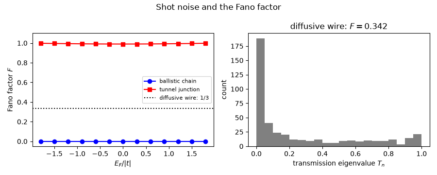
An open channel (\(T_n = 1\)) is noiseless, so a ballistic conductor has \(F = 0\); a tunnel barrier (all \(T_n\ll1\)) has \(F = 1\). Beenakker and Buttiker (1992) showed that a disordered wire in the diffusive regime has the universal \(F = 1/3\): its transmission eigenvalues follow a bimodal distribution, with open and closed channels in a fixed proportion, whatever the material. Steinbach, Martinis and Devoret (1996) and Henny et al. (1999) measured the 1/3.

fano_factor() and fano_factor() compute \(F\) from the singular values of \(\Gamma_{out}^{1/2}G^r\Gamma_{in}^{1/2}\).

import numpy as np
import matplotlib.pyplot as plt
import scipy.sparse as sp

import tbkit.lattices as lattices
from tbkit.kspace import ribbon
from tbkit.plot import Plot
from tbkit.system import System
from tbkit.transport import Transport, RecursiveTransport, lead_from_kspace

t = -1.
rng = np.random.default_rng(2)


def chain(n, weak_link=None):
    lat = lattices.chain()
    lat.get_lattice(n)
    sys = System(lat)
    sys.set_hopping([{'n': 1, 't': t}])
    sys.set_onsite({'a': 0.})
    sys.get_ham()
    ham = sys.ham.toarray()
    if weak_link is not None:
        ham[n // 2, n // 2 + 1] = ham[n // 2 + 1, n // 2] = weak_link
    tr = Transport(ham)
    tr.add_lead([[0.]], [[t]], [[t]], [0])
    tr.add_lead([[0.]], [[t]], [[t]], [n - 1])
    return tr

The lattices

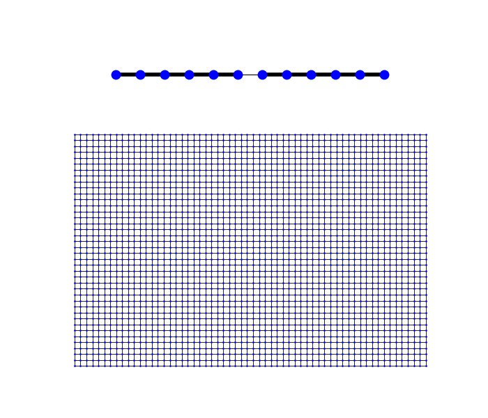
Top: a chain with nearest-neighbour hopping, here with a weak link in the middle (bond widths proportional to the hoppings), as in the tunnel barrier below. Bottom: a square-lattice wire 60 sites long and 40 wide, as in the diffusive wires.

lat_vis = lattices.chain()
lat_vis.get_lattice(12)
chain_vis = System(lat_vis)
chain_vis.set_hopping([{'n': 1, 't': t}])
chain_vis.set_hopping_def({(5, 6): 0.2 * t})
wire = lattices.square()
wire.get_lattice(60, 40)
wire_vis = System(wire)
wire_vis.set_hopping([{'n': 1, 't': t}])
fig_lat, axes_lat = plt.subplots(2, 1, figsize=(7, 6), height_ratios=(1, 5))
Plot(chain_vis).lattice(plt_hop=True, ms=10, c=4., ax=axes_lat[0])
Plot(wire_vis).lattice(plt_hop=True, ms=2, c=0.6, ax=axes_lat[1])

<Figure size 700x600 with 2 Axes>

Ballistic: no noise. A tunnel barrier: Poisson noise.

energies = np.linspace(-1.8, 1.8, 13)
ballistic = chain(20).fano_factor(energies)
tunnel = chain(20, weak_link=0.05 * t).fano_factor(energies)
print('ballistic chain: F <= {:.1e}; tunnel junction: F >= {:.4f}'.format(ballistic.max(), tunnel.min()))
assert np.all(ballistic < 1e-6)
assert np.all(tunnel > 0.98)

ballistic chain: F <= 4.6e-08; tunnel junction: F >= 0.9900

A diffusive wire: one third

Square-lattice wires 40 sites wide and 60 long, with box disorder \(W = 1.6|t|\), conducting through several channels (\(\langle G\rangle \approx 6\,e^2/h\)). The noise and the current are averaged over 20 disorder samples, with the recursive Green’s function.

width, length, disorder, e_f = 40, 60, 1.6, -1.
column = t * (np.eye(width, k=1) + np.eye(width, k=-1))
clean = sp.kron(sp.eye(length), column) + sp.kron(sp.eye(length, k=1) + sp.eye(length, k=-1), t * sp.eye(width))
cols = [list(range(c * width, (c + 1) * width)) for c in range(length)]
strip = ribbon(lattices.square(), [{'i': 0, 'j': 0, 'R': (1, 0), 't': t},
                                               {'i': 0, 'j': 0, 'R': (0, 1), 't': t}], width=width, direction=1)
(h_l, v_l), (h_r, v_r) = lead_from_kspace(strip, -1), lead_from_kspace(strip, 1)
eigenvalues = []
for sample in range(20):
    ham = clean + sp.diags(disorder * (rng.random(length * width) - 0.5))
    wire = RecursiveTransport(ham, cols, (h_l, v_l, t * np.eye(width)), (h_r, v_r, t * np.eye(width)))
    eigenvalues.append(wire.transmission_eigenvalues(e_f))
eigenvalues = np.concatenate(eigenvalues)
fano = np.sum(eigenvalues * (1 - eigenvalues)) / eigenvalues.sum()
print('diffusive wire: <G> = {:.1f} e^2/h, F = {:.3f} (Beenakker-Buttiker: 1/3)'.format(eigenvalues.sum() / 20, fano))
assert abs(fano - 1 / 3) < 0.03
# the bimodal distribution: the eigenvalues pile up near 0 and near 1,
# and are rare in between
open_ = eigenvalues[eigenvalues > 1e-3]
counts = np.histogram(open_, bins=10, range=(0., 1.))[0]
assert counts[0] > counts[-1] > counts[2:8].max()

fig, axes = plt.subplots(1, 2, figsize=(9, 3.6))
axes[0].plot(energies, ballistic, 'o-b', label='ballistic chain')
axes[0].plot(energies, tunnel, 's-r', label='tunnel junction')
axes[0].axhline(1 / 3, color='k', ls=':', label='diffusive wire: 1/3')
axes[0].set_xlabel(r'$E_F / |t|$')
axes[0].set_ylabel('Fano factor $F$')
axes[0].set_ylim(-0.05, 1.1)
axes[0].legend(fontsize=8)
axes[1].hist(open_, bins=20, color='gray')
axes[1].set_xlabel('transmission eigenvalue $T_n$')
axes[1].set_ylabel('count')
axes[1].set_title(r'diffusive wire: $F = {:.3f}$'.format(fano))
fig.suptitle('Shot noise and the Fano factor')
fig.set_layout_engine('tight')

diffusive wire: <G> = 5.6 e^2/h, F = 0.342 (Beenakker-Buttiker: 1/3)