The Anomalous Hall Effect in Real Space: a Disordered Chern Insulator

The Berry-phase theory of the anomalous Hall effect is a statement about Bloch bands, but a real sample has impurities, and no Brillouin zone. The Kubo-Bastin formula needs neither: it is a trace over the whole sample,

\[\sigma_{xy}(\mu) \propto \int d\varepsilon\, f(\varepsilon)\, \mathrm{Tr}\left[v_x\,\delta(\varepsilon-H)\,v_y\,\frac{dG^+}{d\varepsilon} - v_x\,\frac{dG^-}{d\varepsilon}\,v_y\,\delta(\varepsilon-H)\right],\]

which Garcia, Covaci and Rappoport (2015) expanded in Chebyshev polynomials with the kernel polynomial method: tbkit.kpm.hall_conductivity(), with a cost linear in the number of sites.

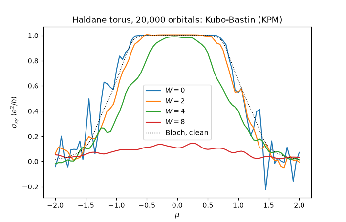
Here: a Haldane model on a torus of 100 x 100 cells (20,000 orbitals), with random onsite energies in \([-W/2, W/2]\). The trace runs over a torus – an open flake would not do, as its edge currents cancel the bulk and the whole trace vanishes in the gap – so the velocities \(v = i[H, \mathbf{r}]\) come from the bond vectors (finite_velocity()), which stay short across the periodic boundary. The quantized anomalous Hall plateau survives disorder stronger than the clean gap, and dies when the disorder is strong enough.

A caveat of the method: its random-vector trace, cheap and accurate in a (mobility) gap, is noisy inside clean bands, where its error falls only as \(1/\sqrt{RN}\) (\(R\) random vectors, \(N\) orbitals). The plateaus are the reliable part of the curves below.

import numpy as np
import matplotlib.pyplot as plt
import scipy.sparse as sparse

import tbkit.kpm as kpm
import tbkit.lattices as lattices
from tbkit.bridges import finite_system
from tbkit.kspace import KSpace
from tbkit.plot import Plot


def haldane(M, t2=0.2):
    '''Haldane model: nearest-neighbour t = 1, i t2 on the second neighbours, mass +-M.'''
    hal = KSpace(lattices.honeycomb())
    hal.set_hopping([{'i': 0, 'j': 1, 'R': R, 't': 1.} for R in [(0, 0), (-1, 0), (0, -1)]])
    for R in [(0, 1), (-1, 0), (1, -1)]:  # a2, -a1, a1 - a2: 120 degrees apart
        hal.set_hopping([{'i': 0, 'j': 0, 'R': R, 't': 1j*t2}, {'i': 1, 'j': 1, 'R': R, 't': -1j*t2}])
    hal.set_onsite({'a': M, 'b': -M})
    return hal


hal = haldane(0.3)
n = 100
ham_clean = hal.finite_ham(n, periodic=True, sparse=True)
vx, vy = hal.finite_velocity(n, periodic=True, sparse=True)
area = n * n * abs(np.linalg.det(np.array(hal.lat.prim_vec)))
n_orb = ham_clean.shape[0]
e_f = np.linspace(-2., 2., 81)
n_moments, n_random = 256, 6

The lattice

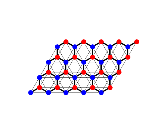
The Haldane model on a patch of \(5\times4\) cells (finite_system()), each bond drawn with a width proportional to its amplitude: the honeycomb lattice’s two sublattices (‘a’ and ‘b’, in two colours), the nearest-neighbour hopping \(t\) (thick) and the complex second-neighbour hoppings \(\pm it_2\) within each sublattice (thin), which break time-reversal symmetry.

fig_lat = Plot(finite_system(haldane(0.3), (5, 4))).lattice(plt_hop=True, ms=12, figsize=(5.5, 4.5))

The clean torus

Without disorder, the torus is the Bloch problem on a 100 x 100 k-mesh, and in the gap \((-0.74, 0.74)\) the KPM value is the Chern number. In the bands it scatters about the Bloch result (hall_conductivity(), dotted) by the noise of the random-vector trace.

_, sigma_clean = kpm.hall_conductivity(ham_clean, vx, vy, n_moments, n_random, e_grid=e_f,
                                                      area=area, seed=0)
bloch = hal.hall_conductivity(e_f, temperature=0.05, nk=n)
chern = hal.chern_number([0], 60)
gap = np.abs(e_f) < 0.5
print('Chern number {:.4f}; clean KPM plateau {:.4f} +- {:.4f}'.format(
    chern, sigma_clean[gap].mean(), sigma_clean[gap].std()))
assert np.allclose(sigma_clean[gap], chern, atol=0.02)

Chern number 1.0000; clean KPM plateau 1.0003 +- 0.0000

Adding disorder

One disorder realization per strength (seeded). At \(W = 2\), wider than the clean gap (1.48), the plateau is intact. At \(W = 4\) the random potential fills the gap with states – the density of states at \(E = 0\) is no longer zero – but these states are localized and carry no current: the plateau survives in a mobility gap. At \(W = 8\), the disorder has destroyed it.

rng = np.random.default_rng(1)
strengths = [0., 2., 4., 8.]
sigma = {0.: sigma_clean}
dos0 = {}
for W in strengths:
    ham = ham_clean + sparse.diags(rng.uniform(-W / 2, W / 2, n_orb))
    if W > 0:
        sigma[W] = kpm.hall_conductivity(ham, vx, vy, n_moments, n_random, e_grid=e_f, area=area,
                                                     seed=0)[1]
    dos0[W] = kpm.dos(ham, n_moments, n_random, e_grid=[0.], seed=0)[1][0] / n_orb
    print('W = {:.0f}: sigma_xy(0) = {:.3f} e^2/h, DOS(0) = {:.4f} per orbital'.format(
        W, sigma[W][np.argmin(np.abs(e_f))], dos0[W]))

centre = np.argmin(np.abs(e_f))
assert abs(sigma[2.][centre] - chern) < 0.03  # the plateau survives W = 2
assert abs(sigma[4.][centre] - chern) < 0.05  # and W = 4...
assert dos0[4.] > 0.01 and dos0[4.] > 100 * dos0[0.]  # ...although states now fill the gap
assert sigma[8.][centre] < 0.5  # strong disorder destroys it

fig, ax = plt.subplots(figsize=(7, 4.5))
for W in strengths:
    ax.plot(e_f, sigma[W], label='$W = {:.0f}$'.format(W))
ax.plot(e_f, bloch, 'k:', lw=1, label='Bloch, clean')
ax.axhline(chern, color='k', lw=0.5)
ax.set_xlabel(r'$\mu$')
ax.set_ylabel(r'$\sigma_{xy}$ ($e^2/h$)')
ax.set_title('Haldane torus, 20,000 orbitals: Kubo-Bastin (KPM)')
ax.legend()

W = 0: sigma_xy(0) = 1.000 e^2/h, DOS(0) = 0.0000 per orbital
W = 2: sigma_xy(0) = 1.005 e^2/h, DOS(0) = 0.0001 per orbital
W = 4: sigma_xy(0) = 0.989 e^2/h, DOS(0) = 0.0366 per orbital
W = 8: sigma_xy(0) = 0.107 e^2/h, DOS(0) = 0.0973 per orbital

<matplotlib.legend.Legend object at 0x10f1e0ec0>